Sue
Sue
Appendix
A.5 Software developed within the work
A.5.1 Sue: a tool for the optimisation of plant functional types.
I adapted the fourth corner method by Legendre et al. (1997) to the task of plant functional grouping. The method is implemented in a Matlab � script. A stand alone version is hosted by the landscape ecology group at the University of Oldenburg.
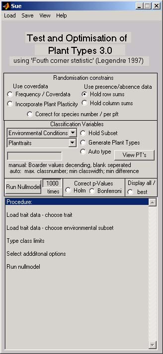
General approach
This program calculates the so called fourth corner statistic. A species � site matrix, a species �trait matrix and an matrix of the environmental conditions at the sites are combined and the occurrence of groups of species in the filed data is compared with that of a null model. The result characterises the response of the species group to an environmental factor. Different data types can be used by choosing different null models. The procedure is also able to optimise functional grouping.
Steps of the analysis
- Load the data
- Chose the null model
- Categorise the species or initialise the automatic categorisation
- Chose environmental factor or factor combination
- Set number of simulations
- Set correction procedure
Functional analysis and modelling of vegetation
- Set Display type (best classification / all classification ; including species)
- Push the <Run Nullmodel> button
- Interpret the result
Manual
1. Load the data
Four files have to be loaded for the analysis. All files have to be tab limited text files. Empty fields are not allowed in the lists. The absence of a species has to be marked with a zero. An additional file containing the plant size is required for one null model.
1.1 |Load | Observational data | ; a species �sites list with frequencies or presence / absence data; no headlines and no species names. All values have to be positive numeric integer values.
1.2 |Load | Trait data | ; a species � trait list listing the measured trait values or categorical variables (e.g. for life cycle) use the dot <.> instead of the comma <,> as decimal marker. A head line (column header) gives the trait names.
1.3 |Load |Environmental data|; a site � factor state list. With a column header naming the factors. While the traits are categorised by the procedure, the environmental factors need to be categorised before. The list must only contain integer values greater than zero. For instance, if the factor pH has to be categorised in values below six, values between six and eight and values above eight, then the column with the column header ‘pH’ consists only of the values 1 (pH<6), 2 (6<pH<8) and 3 (pH>8).
1.4 | Load | Species names | ; a list of the names of the species without column header.
- | Load | Plant size | ; a list of the plant size in number of occupied sub plots by a single plant per site without column header. This file is only required by the null model incorporating plant plasticity. The minimum size is one. Zero values are not allowed.
- Chose the null model Five null models are implemented using different data types and searching for different pattern. For more details of model 2.1.1 and 2.1.2 refer to Numerical
Appendix
Ecology by Legendre et al. 1998, or to chapter three. Null model 2.1.3 is explained in detail in chapter two and null model 2.1.5 in chapter five.
2.1 Presence absence data If frequency data has been loaded, it is transformed to presence absence data by these models.
2.1.1 |Hold row sums| If only the <Hold row sums> radio button is checked, the environmental control model is applied which randomises the entries in the observed matrix in each row, hence the number of sites at which each species occurs remains constant. This model indirectly assumes that the species diversity is similar at each site. If the radio button <Correct for species number / per PFT> is checked, a correction is applied taking a site specific species diversity into account (see chapter three for details).
2.1.2 |Hold column sums| If only the <Hold column sums> radio button is checked, the lottery model is applied which randomises the entries in the observed matrix in each column, hence the species diversity per site remains constant. This model indirectly assumes that the number of sites at which the species occurs is similar for each species. If the radio button <Correct for species number / per PFT> is checked, a correction is applied taking a species specific rarity into account (see chapter three for details).
2.1.3 |Hold row sums| and |Hold column sums| If both radio buttons are checked, the sequential swap procedure is applied maintaining species diversity per site and species rarity. (see chapter three for details).
2.2 Quantitative occurrence data
2.2.1 |Frequency / Cover data | This null model is a version of the sequential swap using abundance data instead of presence absence data. The single records are swaped in a way that the number of records per site and per species remains constant. For instance the following matrix
| 11 | 3 | 10 | 4 |
| 5 | 6 may be swaped to 6 | 5 without changing row or column | |
| sums. | |||
- |Incorporate Plant Plasticity| This null model incorporates a treatment specific plant size. The full procedure or this null model is described in chapter 5.
- Categorise the species or initialise the automatic categorisation Either the response of a single categorisation or of many categorisations can be calculated. If a trait is selected in the pull down menu, a list showing all trait values per species is displayed.
Functional analysis and modelling of vegetation
3.1 Single categorisation: Select the trait to be categorised, in the plant trait pull down menu and type the group limits in the text field below. For instance if the trait ‘plant height’ is selected and the entry in the text field is : | 0 10 15 200 |, than three PTs are formed, the first including all species from height >= 0 and height <=10; the second plant type will be of height > 10 and height < =15 and the last plant type will be of height > 15 and height <=
200. If a syndrome has to be defined, check the | Generate Plant Types| button and proceed by classifying the next trait. If a new trait is chosen (for syndromes), text field will be cleared.
- Automatic categorisation: Select the trait to be categorised in the plant trait pull down menu. Type the three parameter of the automatic classification in the text field below. The first number is the maximum number of trait classes to be formed, the second number is the minimum trait class width, and the last number is the minimum difference between the classifications. Check the auto type button after the first parameter categorisation is filled in the text field. For instance if the parameter | 3 4 3 | are set, than all categorisations with either 1, 2 or 3 trait classes are formed. Each class has a minimum width of 4. All formed classifications are compared with each othe and categorisations, which in which all trait classes are too similar (difference between associated limits below 3) are discarded. All remaining categorisations will be displayed. The automatic classification of several traits can be combined if the |Generate Plant types| radio button is checked.
- Chose environmental factor or factor combination The factors to be included in the analysis can be chosen in the pull down menu. After choosing a factor, the number of sites, number of different treatments and the number of replicates of each treatment is displayed. Combination of factors can be selected by checking the <Hold Subset> button.
- Set number of simulations The number of simulated null communities is set to 1000 by default. The value can be changed by typing a number next to the <Run Nullmodel> button. The smallest possible p-value is one divided by the number of simulations.
- Set correction procedure The p-values may either be corrected using the Holm procedure or the Bonferroni method. By checking one of the checkboxes above the list field. For both methods refer to Numerical Ecology by Legendre et al. 1998.
- Set Display type
Appendix
You can either chose to display all categorisations (required if only a single categorisation is tested), or you may check the display all / best button, to list the best categorisation only. If |View| |Display PFT-species name| is ticked, than the species names for each PFT are displayed.
- Push the <Run> button The analysis may take a while (seconds to days) depending on the number of simulations and the number of different categorisations to be tested. If several categorisations are tested, than each time a categorisation has been finished, its number is displayed either in the MS-DOS window or the Matlab command window.
- Interpret the result After finishing the calculation, the program will display the trait state intervals (Group Intervals) of the grouping, the observed frequencies for each group at sites of each factor combination, the selected factor, the number of sites, the number of treatments, the umber of replicates per treatment, and a factor (factor combination) � PT matrix of the response of the PT to each factor (combination of factors), e.g. the p-values. If syndromes are formed, the PFTs occurring in the data set are listed and the factor � PT matrix is reduced to the PTs which have at least a single occurrence in the data set.
***************************************************************
Copyright by Veiko Lehsten
Landscape Ecology Group (Fac. 5)
University of Oldenburg
PO Box 5634
D-26046 Oldenburg
Germany
Tel. 0049 (0) 441 798 3914
Fax. 0049 (0) 441 798 3914
***************************************************************
Download:
installsue.exe
For a first installation, run the installation file.
It will extract all files to C:\sue\ DONT CHANGE THE DIRECTORY