Chain Pattern: Probabilistic Version of the Hypothetical Syllogism
Chain Pattern: Probabilistic Version of the Hypothetical Syllogism
Keywords
Chain Pattern, Conditional Independence, Hypothetical Syllogism, Model Checking, Theorem Proving, Transitivity of Implication, Cut-Rule, Resolution, Conjunctive Normal Form (CNF), Directed Acyclic Graph (DAG), Generative Probabilistic Model, Joint Probability Mass Function (JPMF), Conditional Probability Mass Function (JPMF), Bayesian Inference, , Bernoulli Random Variable, Bernoulli Distribution, WebPPL, Infer(...), flip(...), condition(...)
Scenario, Proofs, and Mathematical Specification
Background and Motivation
Hypothetical syllogism is an inference rule of classical logic that goes back to Theophrastus. Both premises contain an implication. The conclusion in turn provides an implication (shortening both premises).
If I don't get to the airport in time, I miss my plane.
If I miss my plane, I miss the beginning of the NeurIPS conference.
------------------------------------------------------------------------------------
If I don't get to the airport in time, I miss the beginning of the NeurIPS conference.
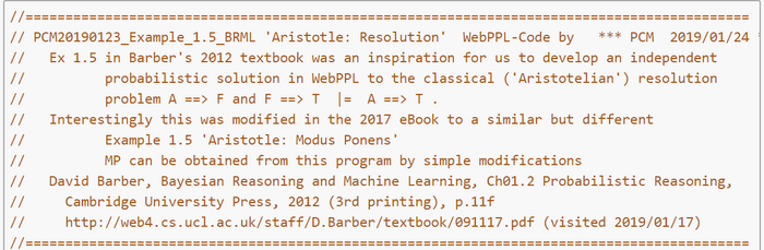
In his textbook Bayesian Reasoning and Machine Learning, Barber presents an introductory example Aristotle: Decision on the Transitivity of Implication (Barber, 2012, p.11, example 1.5). In later electronic editions this example was slightly modified to Aristotle: Modus Ponens. It states: According to logic, the statements "All apples are fruits" and "All fruits grow on trees" lead to the conclusion that "All apples grow on trees". This kind of argumentation is a form of transitivity: From the statements A ⇒ F and F ⇒ T we can conclude from A ⇒ T (Barber, 2016; visited 2019/02/17).
First we describe Barber's example and modify the concepts a little bit, so that they don't prevent transivity. Then we give two semantic proof strategies for the transivity. They are based on model checking (Russell & Norvig, 2016, 3/e, p.249). Models are enumerated and checked whether the syllogistic sentence holds in all models or a negated sentence holds in no model. Next, a syntactic theorem proving strategy is presented. The resolution inference rule is applied directly to the sentence to construct a proof of the desired transivity sentence without checking models (Russell & Norvig, 2016, 3/e, p.249).
In the last paragraph we present our probabilistic version of the hypothical syllogism. We see, that though the antecedents are nonbiased in the case of false premises in the implication this is not true for the inferred implication.
Discussion of Barber's Example 1.5
Barber provides a proof that one can derive from the assumptions
$$P(Fruit = tr | Apple = tr) = P(OnTree = tr | Fruit = tr) = 1$$
and $$ P(OnTree | Apple, Fruit) = P(OnTree | Fruit) $$
the conditional probabilities $$P(OnTree = tr | Apple = tr) = 1.00 $$ and $$P(OnTree = fa | Apple = tr) = 0.00 $$.
This example shows very well which prerequisites must be fulfilled in order to obtain a probabilistic variant of the hypothetical syllogism of classical logic. Above all, the conditional independence of end node T and start node A must be given for a given center node F as formally
$$\left\{T \perp A|F\right\}\equiv P(T|F,A)=P(T|F)$$
Only under this condition the transitivity can be simulated probabilistically. This is only possible with the selected reality section "apples" if the too general concept "fruits" is specialized to "tree fruits". Such a concept specialization is achieved by expanding the intension and/or reducing the extension (Fig. 1).
Thus the random variable in the middle of the syllogism of "isFruit" has to be specialized to "isTreeFruit". Only then can you remove the direct edge from isApple to growsOnTree that prevented transitivity (Fig. 5).
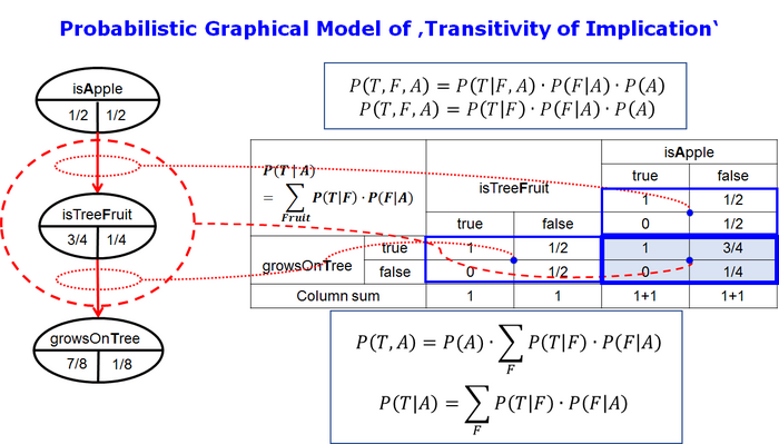
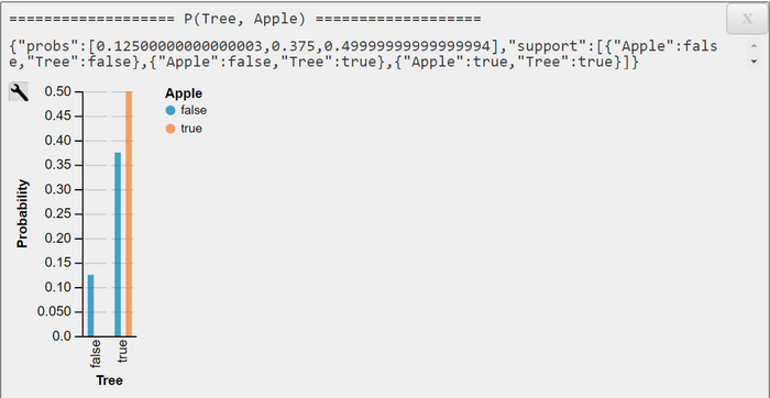
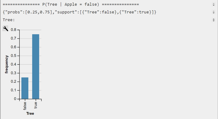
Under this restriction, we are able to replicate the results of Barber. We can also show that $$P(OnTree = true | Apple = false) = 3/4 >> P(OnTree = false | Apple = false) = 1/4 $$.
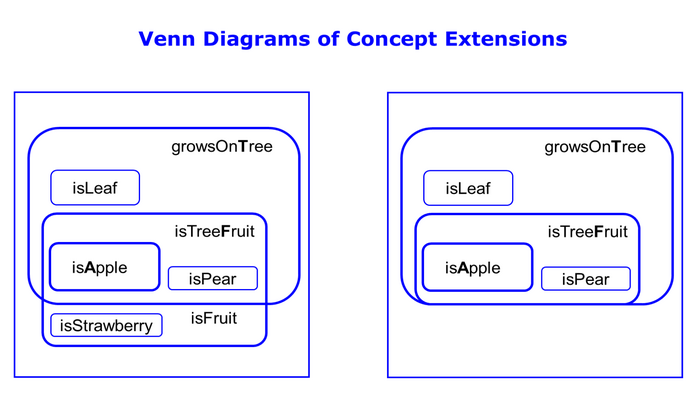
Venn Diagrams of Concept Extensions (Fig 1)
We define a concept as a two-tuple consisting of intention and extension. Intension is the set of predicates or attributes that describe the concept, while extension is the set of objects that belong to the concept. Sometimes it is easier to convey the intention of the concept and sometimes its extension.
For example, it is easier to specify the intention of the concept prime than its extension. On the other hand, it is more difficult to define the concept artwork intentionally than extensionally.
The simplified extensions of the concepts isApple, isFruit and growsOnTree are in Fig. 1 (left). We see at once that isFruit is not suited for the implication isFruit --> growsOnTree because there are fruits which don't grow on trees. So we have to narrow the extension of this concept and add one or more predicates to the intension of isFruit. This way we get the more specialized concept isTreeFruit (Fig 1 - left). The implication isTreeFruit --> growsOnTree is suitable now.
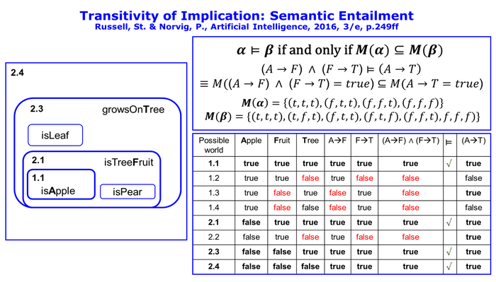
Transitivity of Implications: Proof by Semantic Entailment (Fig 2)
A valuation is an assignment of truth-values to propositional variables (Reeves & Clarke, 1990, p.24). Valuations are sometimes called possible world or models (Fig. 2, columns 1-5). Whereas possible worlds might be thought of as (potentially) real environments that the agent might be or might not be in, models are mathematical abstractions, each of which simply fixes the truth or falsehood of every relevant sentence. ... If a sentence \(\alpha\) is true in a model m, we say that m satisfies \(\alpha\) or sometimes m is a model of \(\alpha\). We use the notation M(\(\alpha\)) to mean the set of all models of \(\alpha\).
Now, that we have a notion of truth, we are ready to talk about logical reasoning. This involves the relation of logical entailment between sentences - the idea that a sentence follows logically from another sentence. In mathematical notation , we write
$$ \alpha \models \beta $$
to mean that the sentence \(\alpha\) entails the sentence \(\beta\). The formal definition of entailment is this:
$$ \alpha \models \beta \text{ if and only if } M(\alpha) \subseteq M(\beta) $$
(Russell & Norvig, 2016, 3/e, p.240).
From Fig 1 we see that
$$ (isApple \rightarrow isTreeFruit) \wedge (isTreeFruit \rightarrow growsOnTree) \models (isFruit \rightarrow growsOnTree) $$.
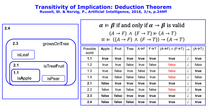
Transitivity of Implications: Proof Using the Deduction Theorem (Fig 3)
The deduction theorem which is a metatheorem states (cf.a. Russell & Norvig, 2016, 3/e, p.249)
$$\text{For any sentences } \alpha \text{ and } \beta, \alpha \models \beta \text{ if and only if the sentence } (\alpha \rightarrow \beta) \text{ is valid} $$ . To this end one only has to build the implication $$\alpha \rightarrow \beta$$ and check its validity. A sentence is valid if it's true in all possible worlds or more abstractly is true in all models. So, we have to check the validity of the derived implication
$$\left( (A \rightarrow F) \wedge (F \rightarrow T) \right) \rightarrow (A \rightarrow T) $$
As can be seen from Fig. 3 this is true, so the transitivity is proven according to this theorem.
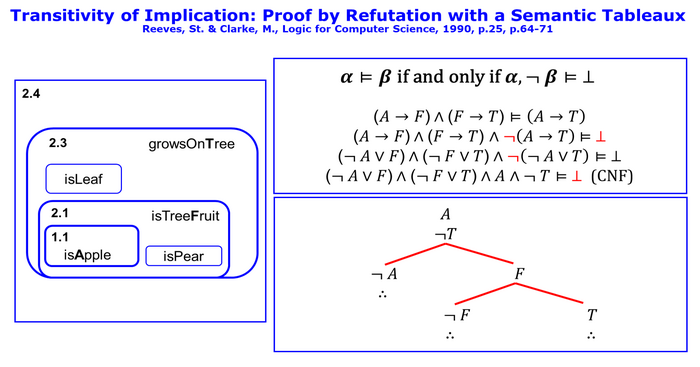
Transitivity of Implications: Proof by Refutation with a Semantic Tableaux (Fig 4)
The semantic tableau is simpler and more expressive than the truth table method. To derive \(\beta\) from \(\alpha\) one negates the conclusion and checks whether it contradicts the premises.
$$ \alpha \models \beta \text{ if and only if } \alpha, \neg \beta \models \perp $$
If it is not possible that the conclusion is wrong with true premises, the conclusion follows semantically from the premises.
The tableau consists of a tree which is formed according to the tableau rules from the expressions of the form \(\alpha, \neg \beta \) . In Fig. 4 we transform our hypothesis
$$ (A \rightarrow F) \wedge (F \rightarrow T) \models (A \rightarrow T) $$ into its negated form
$$ (A \rightarrow F) \wedge (F \rightarrow T) \wedge \neg (A \rightarrow T) \models \perp $$.
The expression left of \(\models\) is transformed in conjunctive normal form (CNF), so that the tree can be constructed according the tableaux rules:
$$ (\neg A \vee F) \wedge (\neg F \vee T) \wedge A \wedge \neg T $$
We only need three rules: the AND rule, the OR rule and the closed path rule (Reeves & Clarke, 1990, p.70; Kelley, 2003, p.50f.). The closed path rule is applied each time the tree is extended by another rule. The Closed-Path-rule looks for inconsistencies in that path. If it detects such an inconsistency it closes the path so that it cannot be extended any further. If all paths in the tree can be closed we have detected a general inconsistency of the negated form so that the hypothesis is semantically valid.
We start with a two-fold application of the AND-rule. This rule takes the two subexpressions of the AND and places them one below the other in the trunk of the tree. Now we have now we have four expressions standing one below the other. Then we apply the OR-rule. At each OR you insert a branch into the tree for each partial expression of the OR. Because the in the left subtree we detect an A and negated A we have a contradiction so that this path can be closed. The right subtree gets expanded only one time with the OR-rule. Then we detect in all paths contradictions, so that every path in the tree is closed.
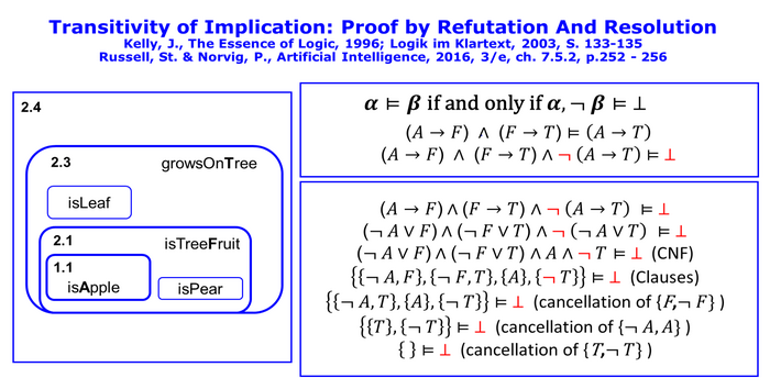
Transitivity of Implications: Proof by Refutation and Resolution (Fig 5)
The resolution rule is a sound and complete inference rule for logical formulas written as conjunctive normal forms (CNFs). The full resolution rule for propositional logic is (Russell & Norvig, 2016, p. 253)
$$ \frac{(l_1 \vee \text{ ... } \vee l_i \vee \text{...} \vee l_k) \wedge (m_1 \vee \text{ ... } \vee m_j \vee \text{...} \vee m_n)} {(l_1 \vee \text{ ... } \vee l_{i-1} \vee l_{i+1} \vee \text{ ... } \vee l_k) \vee (m_1 \vee \text{ ... } \vee m_{j-1} \vee m_{j+1} \vee \text{...} \vee m_n)}$$
where \(l_i \text{ and } m_j\) are complementary literals (i.e., one is the negation of the other). The rule says that it takes two clauses with nonredundant disjunctive literals and produces a new containing all the literals of the original clauses except the two complementary literals. Using set notation for clauses, the resolution rule is more readable for some.
$$ \frac{\left\{ l_1 \text{, ... ,} l_i \text{, ... ,} l_k \right\}, \left\{m_1 \text{, ... ,} m_j \text{, ... ,} m_n\right\}} {\bigl\{ \left\{ l_1 \text{, ... ,} l_i \text{, ... ,} l_k \right\} \backslash \left\{l_i \right\}\bigr \} \cup \bigl\{ \left\{m_1 \text{, ... ,} m_j \text{, ... ,} m_n\right\} \backslash \left\{m_j \right\} \bigr \}}$$
The simplification of the resolvent beneath the horizontal line by applying the set operations of set difference and set union we get
$$ \frac{\left\{ l_1 \text{, ... ,} l_i \text{, ... ,} l_k \right\}, \left\{m_1 \text{, ... ,} m_j \text{, ... ,} m_n\right\}} {\left\{l_1 \text{, ... ,} l_{i-1}, l_{i+1} \text{, ... ,} l_k, m_1 \text{, ... ,} m_{j-1}, m_{j+1} \text{ ... ,} m_n \right\}}$$
Fig 5 shows the necessary steps of the refutation proof by using the resolution inference rule. First we repeat some steps we did in Fig. 4. We transform our hypothesis
$$ (A \rightarrow F) \wedge (F \rightarrow T) \models (A \rightarrow T) $$ into its negated form
$$ (A \rightarrow F) \wedge (F \rightarrow T) \wedge \neg (A \rightarrow T) \models \perp $$.
The expression left of \(\models\) is transformed in conjunctive normal (CNF) and then into clausel form,
$$ (\neg A \vee F) \wedge (\neg F \vee T) \wedge A \wedge \neg T \text{ (CNF) } $$
$$ \left\{ \neg A, F \right\}, \left\{ \neg F, T \right\}, \left\{ A \right\}, \left\{ \neg T \right\} \text{ (set notation) } $$
so that we can apply the resolution rule three times. The result is the empty clause. So the refutation proof showed that the negated form is unsatisfiable. This means that our hypothesis is true.
Probabilistic Graphical Model
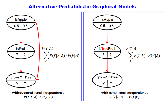
Alternative Probabilistic Graphical Models without or with Conditional Independence (Fig 6)
First we derive the conditional probability mass function (CPMF) $$P(T|A)$$ without further independence assumptions (Fig 6, left). Then we make the conditional independence assumption $$P(T|F,A) = P(T|F)$$ (Fig. 6, right).
According to the directed acyclic graph (DAG) (in Fig 4, left) and the chain rule the joint probability mass function (JPMF) P(T, F, A) is
$$P(T,F,A) = P(T|F,A) \cdot P(F|A) \cdot P(A) $$
The joint marginal P(T, A) is
$$P(T,A) = \sum_{F} P(T|F,A) \cdot P(F|A) \cdot P(A) = P(A) \sum_{F} P(T|F,A) \cdot P(F|A) $$
The CPMF P(T|A) can be obtained by cancellation of P(A)
$$P(T|A) = \sum_{F} P(T|F,A) \cdot P(F|A) $$ (Fig. 6, left).
One can see from P(T | F, A) that the conditional probability is a function of F and A. When we know that an object x is a fruit we cannot predict with certainty that it grows on a tree. We need more information. We need the additional information whether that object is an apple, too.
This is not in the spirit of the transitivity relation. So we have to introduce the conditional independence assumption
$$\left\{T \perp A|F\right\}\equiv P(T|F,A)=P(T|F)$$
At the same time we have to specialize the meaning of the concept or the random variables in the middle layer of the DAG from "isFruit" to "isTreeFruit". Only through this specialization does the model follow the conditional assumption of independence. If we know that an object is a tree fruit, we can predict without additional information that it will grow on a tree.
Under the conditional independence assumption the CPMF P(T|A) simplifies to
$$P(T|A) = \sum_{F} P(T|F) \cdot P(F|A) $$ (Fig. 6, right).
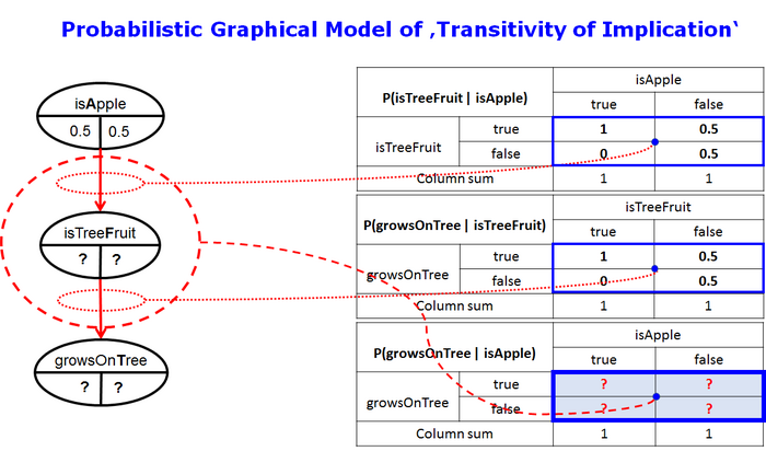
Probabilistic Graphical Model of Hypothetical Syllogism as a Three Node Chain (Fig 7)
Probabilistic Graphical Model of Hypothetical Syllogism as an Inferred Two Node Chain (Fig 8)
WebPPL-Code 'Transitivity of Implication'
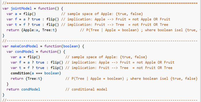
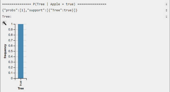
This means that in this closed world apples will certainly grow on trees, while this is true for non-apples only most likely.
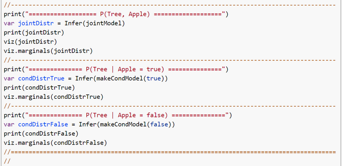
WebPPL-Output JPMF P(Tree, Apple) and Marginals P(Apple), P(Tree)

WebPPL-Output CPMFs P(Tree | Apple = true) and P(Tree | Apple = false)
References and Further Reading
Barber, David. Bayesian Reasoning and Machine Learning, 2012, Cambridge University Press, ISBN-13: 978-0-521-51814-7
Barber, David. Bayesian Reasoning and Machine Learning, 2016; web4.cs.ucl.ac.uk/staff/D.Barber/textbook/091117.pdf (visited 2019/01/19)
Kelly, John. The Essence of Logic, Prentice Hall, 1996, ISBN-13: 978-0133963755
Kelly, John. Logik im Klartext, Pearson Education, 2003, ISBN: 3-8273-7070-1
Pearl, Judea; Glymour, Madelyn, and Jewell, Nicolas P. Causal Inference In Statistics, 2016, Wiley, ISBN: 9781119186847
Pishro-Nik, Hossein. Introduction to Probability, Statistics, and Random Processes, Kappa Research, LLC, 2014, ISBN-13: 978-0990637202
Pishro-Nik, Hossein. Introduction to Probability, Statistics, and Random Processes, www.probabilitycourse.com/ (visited 2019/01/20)
Reeves, Steve & Clarke, Michael, Logic for Computer Science, Addison-Wesley, 1990, ISBN: 0-201-41643-3
Russell, St. & Norvig, P., Artificial Intelligence: A Modern Approach, Pearson EducationLtd, 2016, 3/e, ISBN-13: 978-1292153964