Information and Entropy
Information and Entropy
Entropy, a Measure of Uncertainty
Information Content and EntropyIn information theory \(\textit{entropy}\) is a measure of uncertainty over the outcomes of a random experiment, the values of a random variable, or the dispersion or a variance of a probability distribution \(q\). The more similar \(q\) is to a uniform distribution, the greater the uncertainty about the outcomes of its underlying random variable's values, and thus the \(\textit{entropy}\) of \(q\). In this context, the term usually refers to the Shannon entropy, which quantifies the expected value of the information contained in a message. The formula for information entropy was introduced by Claude E. Shannon in his 1948 paper "A Mathematical Theory of Communication". $$ H_b(X) := E_p[I_b(X)] = - \sum_{j=1}^m p(x_j) \log_b p(x_j)$$
$$p(x_j)$$ is replaced by its surprisal $$\frac{1}{p(x_j)}$$ and the basis \(b\) is set to \(b=2\), the information content \(I_2(x_j)\) of an outcome \(x_j\) is defined to be $$h_2(x_j) = I_2(X=x_j) := \log_2 \frac{1}{p(x_j)} $$ bits (McKay, 2003, p32). The entropy \(H_2(X)\) of the probability mass function (PMF) \(P(X)\) is the expected mean of the Shannon information content $$ H_2(X) := E_p[I_2(X)] = \sum_{j=1}^m p(x_j) \log_2 \frac{1}{p(x_j)} = \sum_{j=1}^m p(x_j) (\log_2 1 - log_2 p(x_j)) $$ $$= \sum_{j=1}^m p(x_j) (0 - log_2 p(x_j)) = \sum_{j=1}^m - p(x_j) log_2 p(x_j) = -\sum_{j=1}^m p(x_j) \log_2 p(x_j), $$ where \(m\) is the number of values or realizations of \(X\). The semantics of \(I_2(X=x_j)\) can be defined as the number of binary Yes/No-questions an omniscient and benevolent agent ('experimenter') is expected to answer so that another questioning agent ('interviewer') can correctly identify the state, value, outcome, or realization xi of the random variable X ('random experiment' hidden from the 'interviewer'). Another verbal statement is "What is the average length of the shortest description of the random variable?" (Cover & Thomas, 2006, p.15) For a \(\textit{uniform}\) PMF H2(X) simplifies to $$ H_2(X) := E_p[I_2(X)] = \sum_{j=1}^m p(x) \log_2 \frac{1}{p(x)} = \frac{1}{m} \sum_{j=1}^m \log_2 m = \frac{1}{m} m \log_2 m = \log_2 m$$ We provide some examples for uniform PMFs in the following table:
The second to last example 'fair 6-sided dice' needs a more detailed explanation. Entropy and Query Strategies \(H_2(X) = log_2 6 = 2.585 \) means that after a random experiment (throw of the fair 6-sided dice) it is expected that the agent has to answer 2.585 yes/no-questions to identify correctly the outcome of the random experiment "throw a fair die" which is the upper side of the die. Because this is an expectation it can be a real number. To guess each outcomes of \(n\) replications of the random experiment "throw a fair die" the total number of yes/no questions needed is expected to be \(2.585 * n\). Because entropy provides us with the expected number of guesses \(H_2(X) = E[I_2(X)]\) the actual number of guesses \(L(x_i)\) falls into the interval between best and worst case: $$ \min_{\rm x_i \in X} L(x_i) \leq E[I_2(X)] \leq \max_{\rm x_i \in X} L(x_i)$$ Queries can be controlled by fixed query strategies (e.g. Fig 1 - 5). The sequence of binary yes/no questions can be mapped to a binary 1/0 code word \(w\). The expected code word length\(E(length(W=w)=: E(WL)\) is greater than or equal to the entropy of the underlying distribution. We present five examples: a linear sequential (Fig 1, Fig 3) and two alternative query strategies (Figs. 2, 4, 5) all controlled by binary trees. Take for example strategy 1 (Fig. 1). To identify \(X = 1\) we need 1 question. Whereas the identification of \(X = 6\) requires 5 questions. The expected word length is \(E(|Wl)=3.333...\) bits. This is also the expected word length \(E(Wl)\) of the variable length prefix code generated by that tree. These are codes with varying length of code words where no shorter word is the prefix of a longer word. In the alternative strategy (Fig. 2) the expected number of questions is with \(2.666...\) bits shorter than the expectation of strategy 1. So this strategy is better than the linear strategy 1 (Fig 1). Of course both \(E(WL)\) are greater than the entropy with \(H_2(X)=2.585\) bits (second to last row in table above). In Fig 3 - Fig 5 we present query strategies for nonuniform PMFs. In Fig 3 and Fig 4 the PMF is \(P(X) = \frac{6-x}{15}\). In this PMF the probability mass is higher the lower value X has. So the linear query strategy (Fig 3) is more optimal than its alternative (Fig 4). The entropy of the PMF is \(H_2(X)= 2.149\) (Fig 3, Fig 4) and the expected word length \(E(Wl)\) of query strategy 1 (Fig. 3) is $$H_2(X)=2.149 < E(Wl) = \left(\frac{5 \cdot 1}{15}+\frac{4 \cdot 2}{15}+\frac{3 \cdot 3}{15}+\frac{2 \cdot 4}{15}+\frac{1 \cdot 5}{15}+\frac{0 \cdot 5}{15}\right) =\frac{35}{15}=2.333... \; bits.$$ The \(E(Wl)= 2.666...\) of the alternative strategy 2 (Fig 4) is higher than that of strategy 1 (Fig 3). So one can see that the optimality of the strategy depends on the underlying PMF. The last example (Fig 5) demonstrates a query strategy controlled by a binary Huffman generated tree (Abelson, Sussman, and Sussman, 1996, ch. 2.3.4, p.163). The query ranges are summarized in Fig 6. The most contrallable query strategy is in Fig 4. Here, the difference between best and worst cases is smallest between all strategies though the overall performance is second to last.
Even the knowledge about the constraint 'values of opposite sides sum to seven' does not reduce the number of necessary questions. Entropy determines an upper bound of the expected information a probability distribution can provide or determines a lower bound on the necessary number of yes/no questions to identify all values of a random experiment controlled by the distribution. This relation between entropy and shortest coding length is a general one. The 'noiseless coding theorem' (Shannon, 1948) states that the entry is a lower bound on the number of bits needed to transmit the state of a random variable (Bishop, 8/e, 2009, p.50). Query games with yes/no questions like "What's My Line?" or "Was bin ich?" have been very popular in the early days of tv. Entropy and the Multiplicity of a System An alternative view of entropy was developed by Boltzman (ca. between 1872 and 1875) in statistical physics. His formulation is $$ S = k* lnW$$ where: \(k\) is a constant and \(W\) is the \(\textit{multiplicity}\) of a system. The multiplicity of a system is a function of the relation between its macro- and micro-states of a system. A tutorial example (HyperPhysics, Georgia State University) should explain the concepts. Entropy and the Log Likelihood of i.i.d. Bernoulli Trials We consider a Bernoulli trial that is a random experiment with binary outcomes \(x \in \{0, 1\}\). This could represent the classical coin-tossing experiment (x=1 for 'head', x=0 for 'tail') or classifications (x=1 for 'class 2', x=0 for 'class 1'). The two probabilities are modelled as \(P(x=1) = p\) and \(P(x=0) = (1-p)\). The probability distribution over \(X\) can be written as $$P(X) := p^x(1-p)^{1-x} = p^{[x=1]}(1-p)^{[x=0]}$$ where '[...]' are the Iversen bracket operators. If we have a set \(D = \{x_1, ..., x_n\}\) of \(n\) independently drawn \(x_i\) we can construct the likelihood of the data set \(D\) conditional on \(p\) $$ L(D|p) := \prod_{i=1}^n p^{[x_i=1]}(1-p)^{[x_i=0]}.$$ The log-likelihood \(l(D|p)\) is $$ \log L(D|p) = l(D|p) := \log p \sum_{i=1}^n [x_i=1] + \log(1-p) \sum_{i=1}^n [x_i=0].$$ Because the maximum likelihood estimator \(p_{ML}\) of \(p\) is (Bishop, 2009, p.69) $$ p_{ML} = \frac{1}{n} \sum_{i=1}^n x_i $$ we can rewrite the log-likelihood as $$ l(D|p) := \log p \cdot n \cdot p_{ML} + \log(1-p) \cdot n \cdot (1- p_{ML}).$$ the conditional estimators are in the limit equal to its parameters, or $$ \lim_{n \to \infty} \sum_{i=1}^n [x_i=1] = n \cdot p$$ and $$ \lim_{n \to \infty} \sum_{i=1}^n [x_i=0] = n \cdot (1-p) $$ the log likelihood is $$ \lim_{n \to \infty} l(D|p) = \log p \cdot n \cdot p + \log(1-p) \cdot n \cdot (1-p).$$ Now, when we rename \(p_1 := p\) and \(p_2 := (1-p)\) the log-likelihood can be written as a compact expression $$ \lim_{n \to \infty} l(D|p) = n \sum_{j=1}^2 p_j \log p_j.$$ We see that (at least for Bernoulli distributions) \(\textit{entropy}\) is equal to the \(\textit{negative expectation of the log-likelihood}\) (here both measured in bits) $$ H_2(X) = E[l_2(D|p)] := - \lim_{n \to \infty} \frac{l_2(D|p)}{n}$$ where $$ \lim_{n \to \infty} l_2(D|p) = n \sum_{j=1}^2 p_j \log_2 p_j.$$ This relation will be important, when we study cross-entropy and the cross-entropy error function. Entropy and the Log Likelihood of i.i.d. categorical trials The multicategorical distribution is an extension of the Bernoulli distribution with binary support \(x \in \{0, 1\}\) to a distribution with multicategorical support \(x \in \{1, 2, ..., k\}\). It can be used e.g. to model a throw of a dice or a game of roulette. The probability mass function (pmf) is $$P(x=i|p) = p_i$$ or $$P(X=x) = p_1^{[x=1]} \cdot ... \cdot p_k^{[x=k]} = \prod_{j=1}^k p_j^{[x=j]}.$$ The likelihood L(D|p) is $$ L(D|p) := \prod_{i=1}^n \prod_{j=1}^k p_j^{[x_i=j]}$$ and the log-likelihood \(\log L(D|p) = l(D|p)\) $$ l(D|p) := \sum_{i=1}^n \sum_{j=1}^k [x_i=j] \log p_j.$$ The index \(i\) does not contain information so we can simplify the summation $$ l(D|p) := \sum_{j=1}^k \sum_{i=1}^n [x=j] \log p_j.$$ The inner sum over \(i\) is the frequency \(n_j\) of category \(j\) which is \(n\) times the maximum likelihood estimator \(p_{j_{ML}}\) of \(p_j\) $$ \sum_{i=1}^n [x=j] = n_j = n \cdot p_{j_{ML}}.$$ In the limit \(n_j\) is equal to \(n \cdot p_j\) $$ \lim_{n \to \infty} \sum_{i=1}^n [x=j] = n_j = n \cdot p_j$$ so the log-likelihood can be further simplified to $$ \lim_{n \to \infty} l(D|p) := \lim_{n \to \infty} \sum_{j=1}^k n_j \log p_j = \sum_{j=1}^k n \cdot p_j \log p_j $$ $$ = n \sum_{j=1}^k p_j \log p_j$$ Even for the categorical distribution \(\textit{entropy}\) is equal to the \(\textit{negative expectation of the log-likelihood}\) (here both measured in bits) $$ H_2(X) = E[l_2(D|p)] := - \lim_{n \to \infty} \frac{l_2(D|p)}{n} = - \sum_{j=1}^k p_j \log_2 p_j$$ where $$ \lim_{n \to \infty} l_2(D|p) = n \sum_{j=1}^k p_j \log_2 p_j.$$ The relation between entropy and log-likelihood is also important, when we study cross-entropy and the cross-entropy error function. References Abelson, H., Sussman, G.J., & Sussman, Julie, Structure and Interpretation of Computer Programs, Cambrige, MA: MIT Press, 1996, 2/e - the 'bible' of schemers, lays the foundation for functional probabilistic programming languages like CHURCH, WebCHURCH, and WebPPL ; provides a chapter on Huffman codes - Bishop, Christopher M., Pattern Recognition and Machine Learning, Heidelberg & New York: Springer, 8/e, 2009 - an early standard reference for machine learning - Dümbgen, Lutz, Stochastik für Informatiker, Heidelberg-New York: Springer, 2003 - Stochastic theory written by a mathematical statistician (unfortunately only in German) with some examples from CS (eg. entropy, coding theory, Hoeffding bounds, ...) - Fraundorf, P., Examples of Surprisal, www.umsl.edu/~fraundorfp/egsurpri.html, (2021/03/30) MacKay, David J.C., Information Theory, Inference, and Learning Algorithms, Cambridge University Press, 2003, www.inference.org.uk/itprnn/book.pdf (visited, 2018/08/22) - The view of a well respected and authorative (see e.g. Pearl, 2018, The Book of Why, p.126) physicist on early Bayesian machine learning, coding theory, and neural nets; interesting how a physicist treats stochastics - Shannon, C. E., A Mathematical Theory of Communication. Bell System Technical Journal, 1948, 27: 379-423, 623-656. - This paper was the birth of information theory - Wikipedia, Entropy, (2021/04/08) Wikipedia, Information content, (2021/03/30) Wikipedia, Iverson bracket, (2021/04/6) Wikipedia, Was bin ich ?, (2021/03/21) Wikipedia, What's My Line ?, (2021/03/21) Wikipedia, Categorical distribution, (2021/04/07) | |||||||||||||||||||||||||||||||||||||||||||||||
----------------------------------------------------------------------------------- This is a draft. Any feedback or bug report is welcome. Please contact: | |||||||||||||||||||||||||||||||||||||||||||||||
| claus.moebus@uol.de | |||||||||||||||||||||||||||||||||||||||||||||||
| ----------------------------------------------------------------------------------- |


WebPPL Code
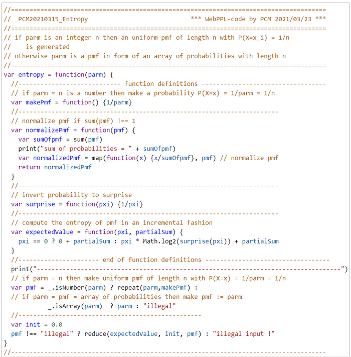
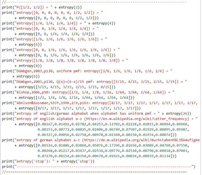
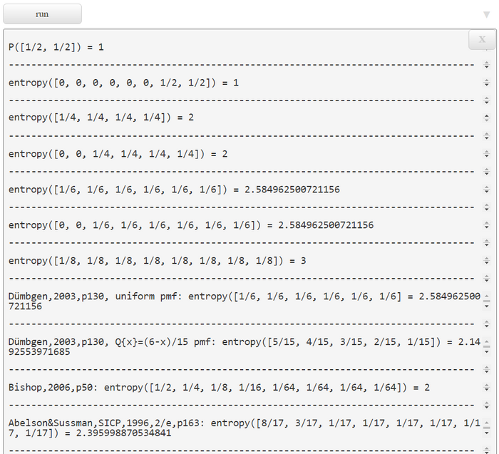
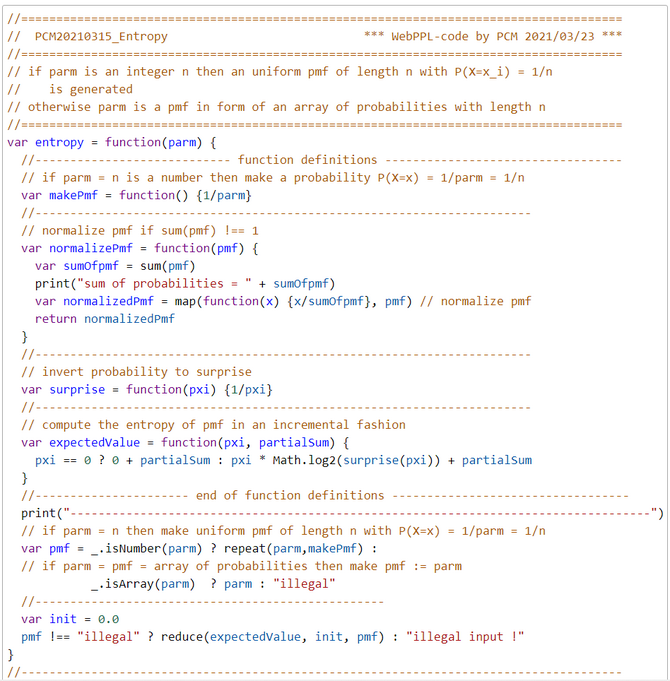
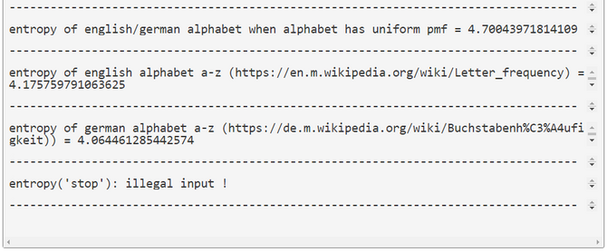
This code snipped should give an impression how's the look and feel of WebPPL. WebPPL is a pure functional DSL embedded in JS. The only imperative constructs are definitions with the keyword \(\textit{var}\). The definition \(\textit{var}\) is a bit misleading, it should be better substituted by the JS-keyword \(\textit{const}\) or the SCHEME-keyword \(\textit{define}\) to make it clear that only a constant or a function are defined. In this WebPPL-snippet lodash functions \(\textit{_.isNumber}\) and \(\textit{_.isArray}\) are used but no advanced WebPPL-inference features. Like in any other functional language there are no loops. Instead e.g. sums and expectations are computed by the \(\textit{sum}\) and \(\textit{reduce}\) functions. In the last three function calls we computed the entropy of three PMFs with the alphabet a-z. The first entropy is based on the assumption that the PMF is uniform. The entropy is \(E(I_2(X)=4.7 bits\). This means that it is expected that we need approximately 5 guesses to correctly identify a letter hidden from us. With the next two function calls of \(\textit{entropy}\) we computed the entropy of the english and the german alphabet's PMFs \(E(I_2(X_{english})=4.176 bits\) and \(E(I_2(X_{german})=4.064 bits\). This shows that German is better predictable than English, at least at the level of individual letters. References Wikipedia, en.m.wikipedia.org/wiki/Letter_frequency , (2021/03/22) Wikipedia, de.m.wikipedia.org/wiki/Buchstabenh%C3%A4ufigkeit, (2021/03/22) ----------------------------------------------------------------------------------- This is a draft. Any feedback or bug report is welcome. Please contact: |
| claus.moebus@uol.de |
| ----------------------------------------------------------------------------------- |


Exercises
The basic WebPPL-code for the exercises can be found here as a PCM20210315_Entropy.js file. You can copy the file's content into the WebPPL-box and run the file in the browser.
1. Replace the \(\textit{reduce}\)-function call in the WebPPL-script by a call of the WebPPL-library-function \(\textit{sum}\).
2. Replace all calls the WebPPL-library-functions \(\textit{sum, reduce}\) by function calls of selfdefined functions.