Continuous-Time Discrete-State Stochastic Decay
Continuous-Time Discrete-State Stochastic Decay
Continuous-Time Markov Chain of Degradation, Decay, or Departure
Introduction
A simple homogeneous degradation, decay (e.g. memory decay), death, or departure process can be described as a directed graphical model (stoichiometric equation in chemics):
$$ N_A \stackrel{\lambda}{\longrightarrow} {\varnothing} \; \; \; \qquad (1)$$
where:
$$ A \text{ := is a species of interest} $$
$$ N_A \text{ := is the number of particles of species of interest} $$
$$ \lambda \text{ := is the rate constant of degradation events} $$
$$ \varnothing \text{ := is a species of no special interest} $$
In a homogeneous process the rate is defined as a constant $$\lambda$$ so that $$\lambda \cdot dt $$ gives the probability that a randomly chosen particle of A reacts, degrades, dies, decays, or departs during the time interval $$[t, t + dt) $$ where t are time and dt an (infinitesimally) small time step.
In an in- or nonhomogeneous process the rate is dependent on time or state $$\lambda(t) \text{ or } \lambda(N_A(t)) $$ so that $$\lambda(t) \cdot dt \text{ or } \lambda(N_A(t)) \cdot dt $$ gives the probability that a randomly chosen particle of A reacts, degrades, dies, decays, or departs during the time interval $$[t, t + dt) $$ where t are time and dt an (infinitesimally) small time step.
The stoichiometric equations or the DAGs are now:
$$ N_A \stackrel{\lambda(t)}{\longrightarrow} {\varnothing} \; \; \; \;\text{ with time-dependent rate } \qquad (2.1)$$
$$ N_A \stackrel{\lambda(N_A)}{\longrightarrow} {\varnothing} \; \; \; \text{ with state-dependent rate } \qquad (2.2)$$
The Definition of the (In-)Homogeneous Counter Decay Process
The "naive" implementation of the solution of the decay counter process is based not on dt but on a discrete approximation $$\Delta t >> dt$$ so it is wise to reuse and modify the second definition of the Poisson process. The decay process $$N_A(t), t \in [0, \infty)$$ is called a homogeneous counter decay process with rate $$\lambda > 0 $$ if all of the following conditions hold:
$$1. \;\;N_A(0) = N_{A_0} > 0\; \; \text{ ; } $$
$$2. \;\;N_A(t) \text{ has independent and stationary increments} $$
then we have
$$P(N_A(\Delta t) = 0) \approx 1 - \lambda \Delta t \qquad (3.1.1)$$
$$P(N_A(\Delta t) = -1) \approx \lambda \Delta t \qquad (3.1.2)$$
$$P(N_A(\Delta t) = -2) \approx 0 \qquad (3.1.3)$$
or more precisely
$$P(N_A(\Delta t) = 0) = 1 - \lambda \Delta t + o(\Delta t) \qquad (3.2.1)$$
$$P(N_A(\Delta t) = -1) = \lambda \Delta t + o(\Delta t) \qquad (3.2.2)$$
$$P(N_A(\Delta t) = -2) = o(\Delta t) \qquad (3.2.3)$$
where "little o" denotes a function g(.) $$ o(\Delta t) := g(\Delta t) $$ that 'vanishes' faster than $$\Delta t $$ when
$$ \lim_{\Delta t \to 0} \frac{g(\Delta t)}{\Delta t} = 0, \qquad (4) $$
or short
$$ o(\Delta t) \rightarrow 0 \text{ as } \Delta t \rightarrow 0 \; \; .$$
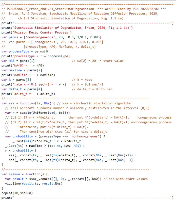
WebPPL-Script: Stochastic Simulation of (In-)Homogeneous Process with Constant Time Increment Delta
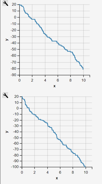
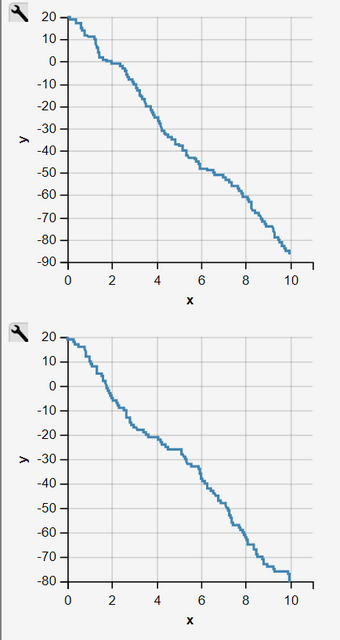
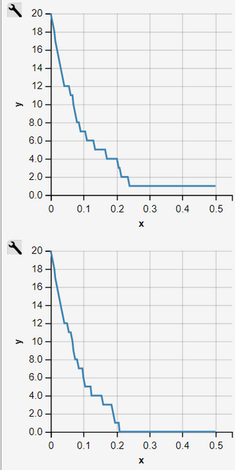
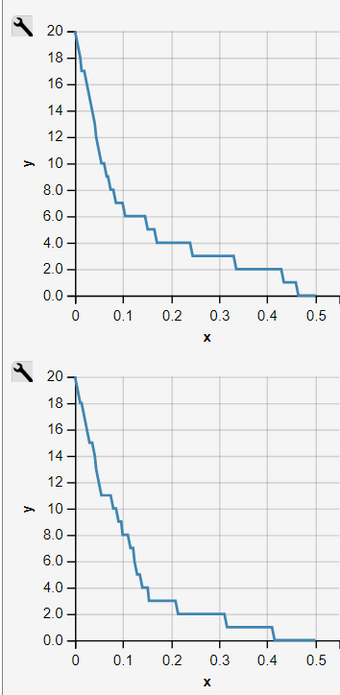
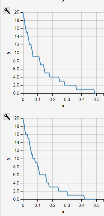
Simulation Runs as an Inhomogeneous Pure Decay Process
Fig. 1: Parameters of Inhomogeneous Process with State-dependent Rates
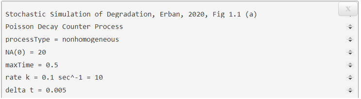
Fig. 2 - 11: Sequence of 10 Independent Simulation Runs of an Inhomogeneous Pure Decay Process
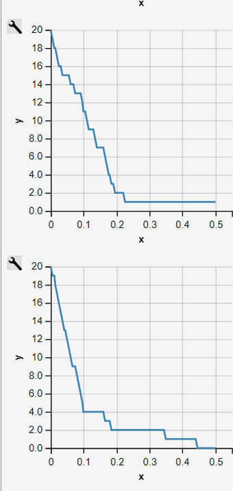
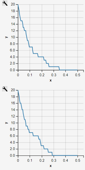
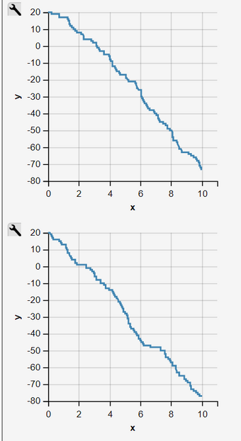
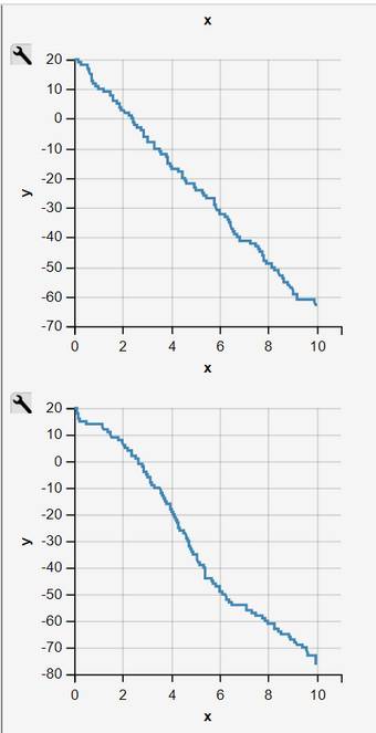
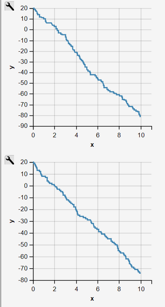
Simulation Runs as an Homogeneous Pure Decay Process
Fig. 1: Parameters of Homogenous Process
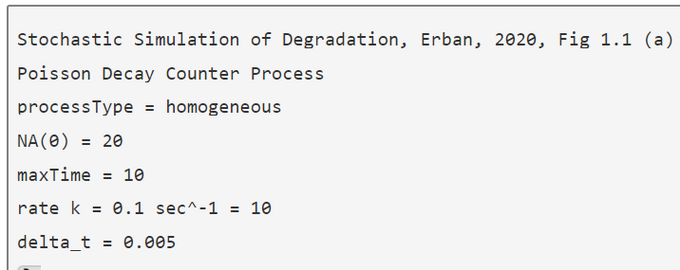
Fig. 2-11 Independent Runs