BCM-Ch06.1: Latent Class Model "Exam Scores"
BCM-Ch06.1: Latent Class Model "Exam Scores"
BCM 'Exam Scores' Model for Two Latent Classes
Lee & Wagenmakers (Bayesian Cognitive Modeling, 2013, ch. 6.1, p.77-78) file this model under Latent-mixture models without proper definition of this term and without making it evident where the mixing takes place. We think that the label Latent-Class is more appropriate than Latent-Mixture for the Exam Scores model.
"A mixture model, ..., usually means that each individual data point y(i) is assumed drawn from one of a list of possible distributions. This can be considered as a clustering of the points into groups G(j) (j=1,...,J), where y(i) is a member of group T(i) and has a distribution parameterised by theta(T(i)). We may write this general model as
y(i) ~ p(y(i) | theta(T(i)), G(T(i)), T(i) ~ Categorical(p[])
so that the probability that y(i) is in the jth group G(j) is PR(T(i)=j)=p(j)." (Lunn et al., The BUGS Book, 2013, p.280f)
In this vague sense the Exam Scores model is a latent mixture model, but the data in this application are assumed not to be generated by a mixture of distributions but by a set of mutual exclusive classes with according latent parameters: group membership probabilities are discrete values {0,1}. So the label Latent-Class seems to be more appropriate for the Exam Scores model.
The task in its original wording: "Suppose a group of 15 people sit an exam made up of 40 true-or-false questions, and they get 21, 17, 21, 18, 22, 31, 31, 34, 34, 35, 35, 36, 39, 36, and 35 right. These scores suggest that the first 5 people were just guessing, but the last 10 had some level of knowledge.
One way to make statistical inferences along these lines is to assume there are two different groups of people. These groups have different probabilities of success, with the guessing group having a probability of 0.5, and the knowledge group having a probability greater than 0.5. Whether each person belongs to the first or the second group is a latent or unobserved variable that can take just two values. Using this approach, the goal is to infer to which group each person belongs, and also the rate of success for the knowledge group." (Lee & Wagenmakers, 2013, p.77)
The probabilistic graphical model and the Bugs/Jags code are presented below. Discrete variables are designated by square nodes, continous by circle nodes. White nodes are latent and have to be inferred. Grey nodes are manifest; either observed data or set as constants. Single bordered nodes are stochastic and double bordered are deterministic derived variables.
The symbols denote:
(1) n = #questions (here set to n = 40)
(2) k(i) = #right or correct answers of person i
(3) psi = ability parameter of the guessing group (here set to 0.5)
(4) phi = ability parameter of the knowledge group (constrained to be between 0.5 and 1.0)
(5) z(i) = group membership of person i (is either 0 or 1; 0 is guessing group)
(6) theta(i) = ability parameter of person i
The only row of code which could be interpreted as a kind of mixing ist the fourth line from below:
theta[i] <- equals(z[i],0)*psi+equals(z[i],1)*phi.
But this is not true, because the semantics of this BUGS line-of-code is a conditional expression. Because BUGS does not know IF-THEN-ELSE constructs, conditional expressions have to be simulated by indicator functions (e.g. equal(X, Y)):
equal (X, Y) means IF(X == Y) THEN 1.
So the meaning of the above line-of-code is (translated to R):
theta[i] <- if(z[i] == 0) psi else phi.
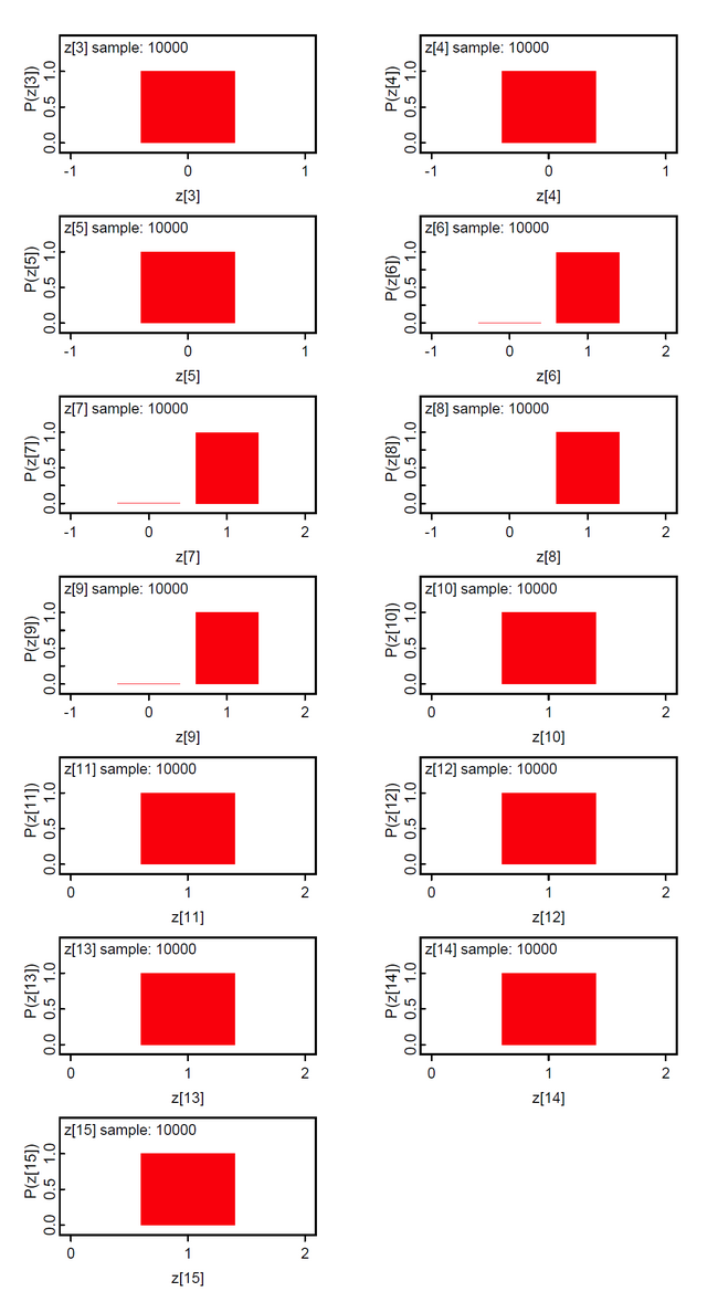
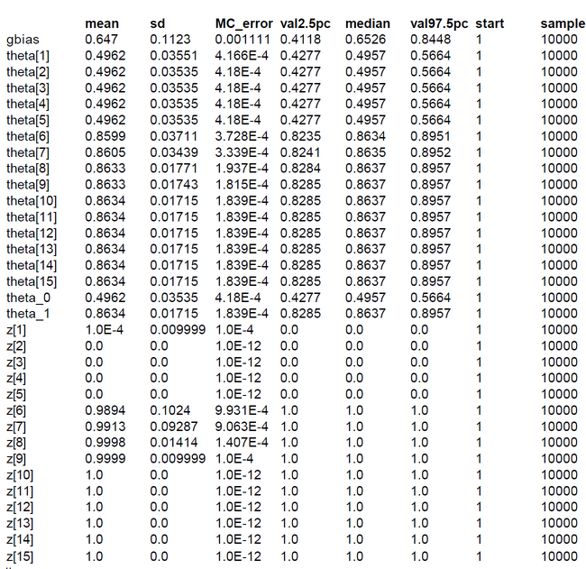
Plot and summary below show that the 95%-posterior-high-density region of the phi-parameter is 0.828-0.894. Furthermore the latent class indicator z indicates the class membership without any error. This is not astonishing because the Exam Scores problem is similar to hiding and looking for easter eggs because the data were constructed according to the hypothesis that there should be the two classes guessers and knowers.


Modified BCM Exam Scores Model for Two Latent Classes
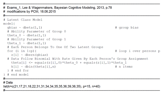
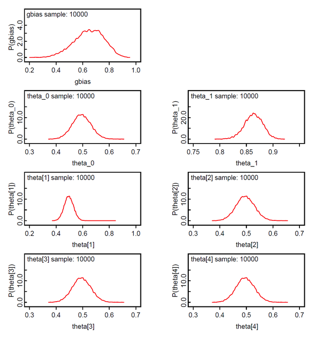
We modified the Lee & Wagenmakers model in various ways: (1) We introduced a bias parameter gbias for estimating the group size, (2) both group-specific ability parameters theta_0 and theta_1 are unconstrained; their priors are uniform flat with dbeta(1,1), and (3) we use only one for loop running over persons.
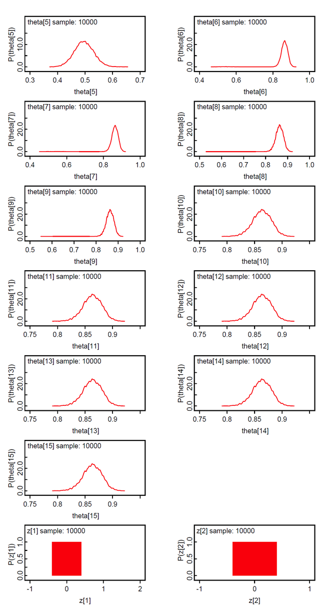
We ran the simulation with OpenBUGS. 10000 samples with thinning=10. The results show that the knowledge group 1 has an estimated sizeof 64.7% (mean of gbias = 0.647). The ability of the guessing group is the mean of the posterior theta_0; which is 0.4962. The ability of the knowledge group is 0.8634. All 15 class memberships could be inferred correctly.
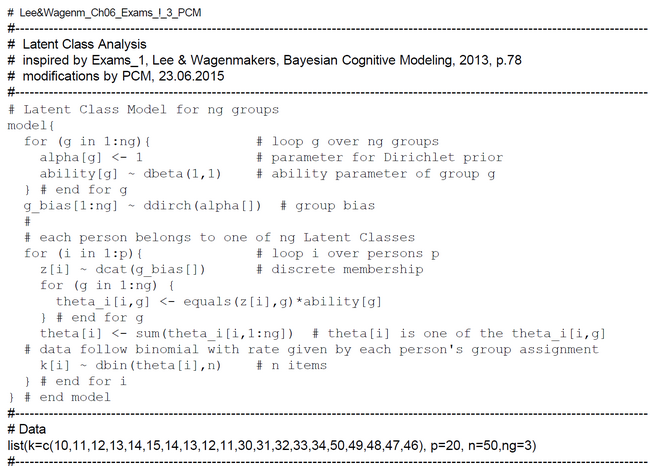
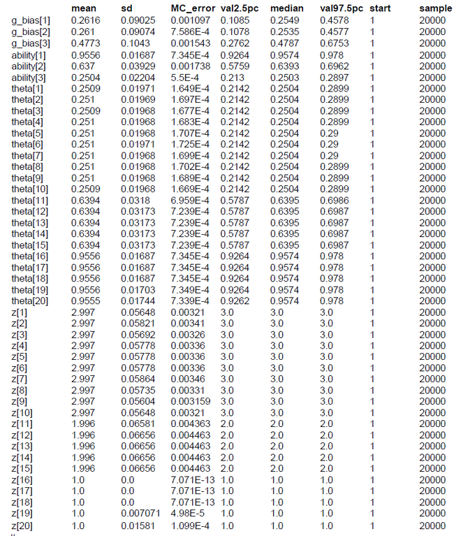
Latent Class Model for G Classes of Binomial Distributed Variables
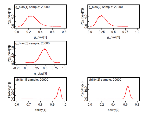
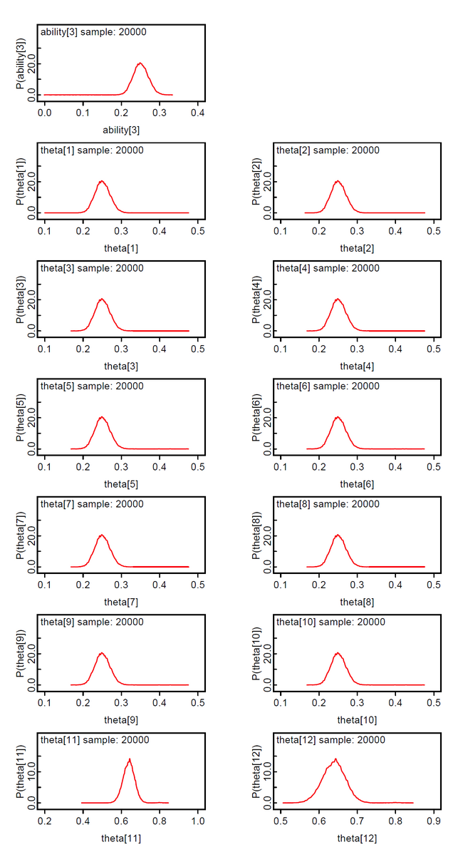
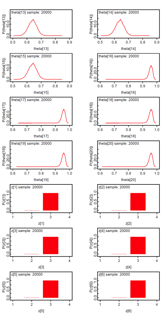
In this model the priors of the class membership g_bias[] are sampled from the Dirichlet distribution with hyperparameter alpha[] = 1. This means that we assume equal probable class memberships. The class membership indicators z[i] are discrete from the set {1,2,...ng} and the theta[i] are not the expected mean of the group-specific theta[i,g] but selected from the set {theta[i,1], theta[i,2], ..., theta[i, ng]}.
The results show that persons 1-10 with scores 10-15 constitute the 3rd latent class; accordingly persons 11-15 with scores 30-34 the 2nd latent class, and persons 16-20 with scores 46-50 the 1st latent class. We suspect that the method is not very discriminative. We found that the z[i] will loose their discrete nature with data having smaller between group variance.