BCM-Ch04.1: Inferring a mean and a Standard Deviation
BCM-Ch04.1: Inferring a mean and a Standard Deviation
BCM-Ch04.1: OpenBUGS-Code for 'Inferring a Mean and Standard Deviation'
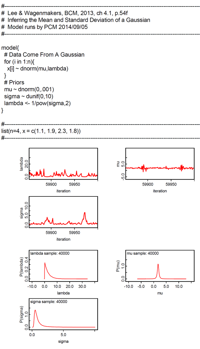
"One of the most common inference problems involves assuming data following a Gaussian (also known as a Normal, Central, or Maxwellian) distribution, and inferring the mean and standad deviation of this distribution from a sample of observed independent data. The mean of the Gaussian is mu and the standard deviation is sigma. WinBUGS parameterizes the gaussian distribution in terms of the mean and precision, not the mean and variance or the mean and standard deviation. These are all simply related, with the variance being sigma^2 and the precision being lambda = 1/sigma^2." (Lee & Wagenmakers, 2013, p.54) BUGS contains an abstract simple functional modeling language with restricted expressiveness (e.g.: an IF and recursion is lacking). Furthermore the sampling process is rather opaque. So BUGS appears to be an abstract 'black box'. Many mathematical details are hidden from the user. This can be helpful for people with mathphobia. For others it is irritating. One example is the 'for-loop' in this examples BUGS code. Intuition tells us that this should compute the likelihood. The code within this 'for-loop' is ( x[i] ~ dnorm(mu, lambda) ). What is the meaning of the tilde '~' ? "In statistics, the tilde is frequently used to mean 'has the distribution (of),' for instance,  means 'the stochastic (random) variable
  has the distribution
  (the standard normal distribution)." (Acklam, Peter and Weisstein, Eric W. "Tilde." From MathWorld--A Wolfram Web Resource. mathworld.wolfram.com/Tilde.html ). We think that this is the declarative semantics of '~'. In the context of simulations as in BUGS there is obviously a second kind of semantics. We call it operational semantics: X or x is sampled from the distribution. Both interpretations are consistent for the priors of mu and sigma. If we consult the official BUGS book we find this: 1. The tilde '~' "... represents (a) stochastic dependence. The left-hand side of a stochastic statement comprises a stochastic node, and the right-hand side comprises a distribution ... Stochastic nodes are variables that are given a distribution ... may be observed and so be data, or may be unobserved and hence be parameters, which may be unknown quantities underlying a model, censored (partially observed) observations, or simply missing data." (LUNN et al., The BUGS Book, 2013, p.21). This is due to its context dependence rather vague. 2. The tilde '~' "... means 'is distributed as' and denotes a stochastic relation;" (LUNN et al., The BUGS Book, 2013, p.329). This is also rather vague, if the tilde appears in the model code. What kind of semantics is true for "x[i] ~ dnorm(mu, lambda)" ? If the declarative semantics is true, then x[i] ~ prior-distributions. The next question is, how do I get the posterior P(mu, sigma | x-data) ? In the model code the symbols mu and sigma denote only priors. If the operational semantics is true the code line "x[i] ~ dnorm(mu, lambda)" suggests that x[i] is sampled from a Gaussian distribution. But this is problematic, because the sampled x[i] would nearly never be equal to the corresponding datum x[i], in the case of floating point numbers. Instead we expect that the likelihood L( x[i] | mu, lambda is calculated ) within the for-loop. That is conceptionally very different from a sampling "x[i] ~ dnorm(mu, lambda)". What is also disturbing is the fact that the priors and posteriors are represented by the same symbols in the code and the monitor windows in the GUI which show the plots of the poseterior pdfs. We believe that the modeling approach within WebCHURCH could be more transparent.
BCM-Ch04.1: CHURCH-Code for Rejection-Based Sampling when "Inferring a mean and a standard deviation"
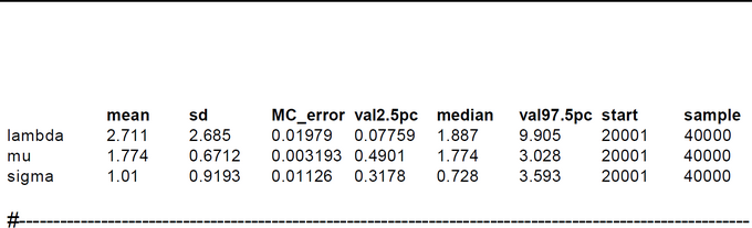
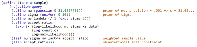
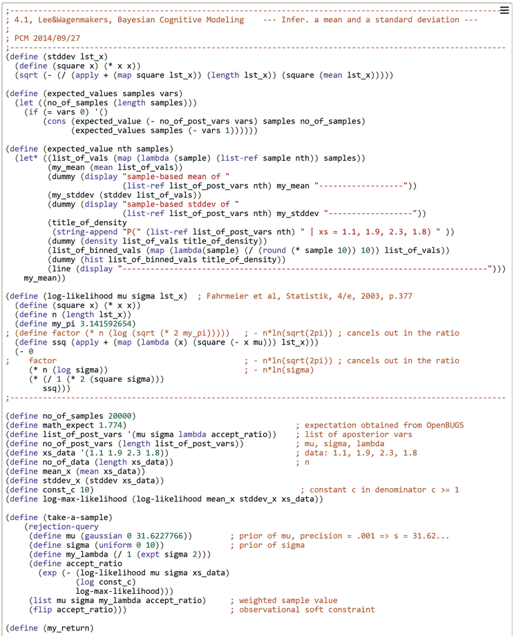
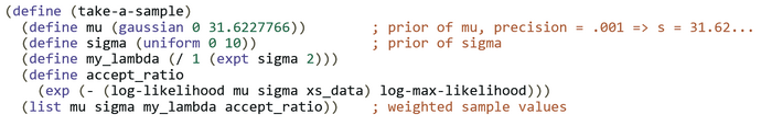
We want to study what kind of models could be developed in WebCHURCH. The WinBUGS-code from Lee & Wagenmakers is translated by us to a functional WebCHURCH program.The generative model is contained in the CHURCH function 'take-a-sample'. This code of this function should be equivalent to the model{...}-part of the OpenBUGS program.
"In the situation where the posterior distribution is not a standard functional form, rejection sampling with a suitable choice of proposal density provides an alternative method for producing draws from the posterior. Importance sampling and sampling importance resampling (SIR) algorithms are alternative general methods for computing integrals and simulating from a general posterior distribution."(Albert, J., Bayesian Computation with R, 2009, 2/e, p.87f).
Up to now rejection-based sampling enforced in our programs a binary decision whether to accept a sample or not. This is based on the fullfillment of a hard observational constraint. Now, in a kind of ‘Soft-Rejection-Based Sampling’ this decision is based on a Bernoulli experiment with an evidence-based bias ('acceptance probability'). Thus the decision is dependent on a soft constraint - the acceptance ratio -.
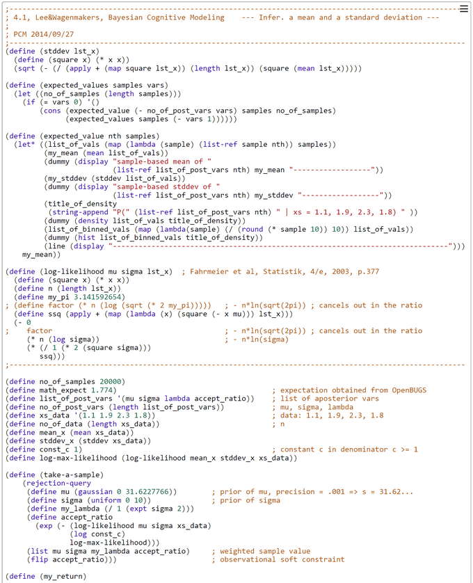
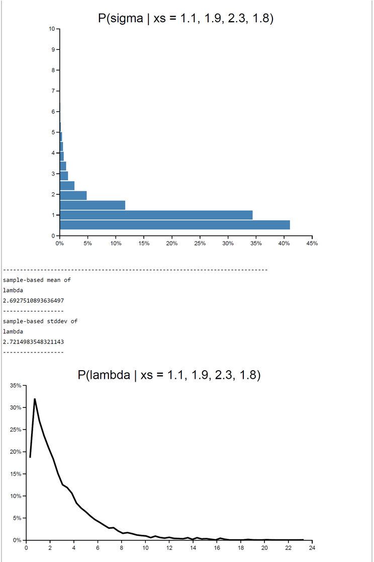
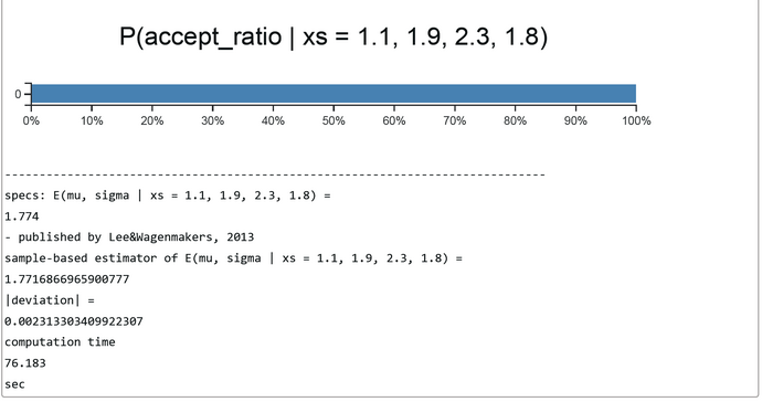
In this case 'take-a-sample' contains the code for an adaptive 'acceptance-ratio' which is equal to the probability of acceptance for this special sample. The P(Acceptance) = [ L(x1,...,xn | mu ~ N(0, sqrt(1000), sigma ~ U(0, 10)) / c*L(x1,...,xn | mu = x-bar, sigma = s) ]= exp[ ln L(x1,...,xn | mu ~ N(0, sqrt(1000), sigma ~ U(0, 10)) - ln c*L(x1,...,xn | mu = x-bar, sigma = s)]. The value of the constant c >= 1 controls the expected value E(P(Acceptance)). Its default value is 1.
In 'take-a-sample' the probability of acceptance is a function of the difference of two log-likelihoods. The likelihood in the numerator is a function of the prior-sampled mu and sigma, the likelihood in the denominator is a constant and is based only on the sample-estimates x-bar and s. This likelihood is the maximum-log-likelihood. If c=1, the sampled mu and sigma are identical to x-bar and s. Then the difference of the log-likelihoods is zero, and the probability of acceptance is P(acceptance) = exp(difference) = exp(0) = 1.
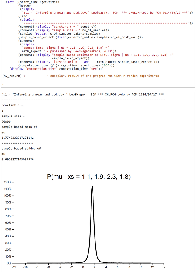
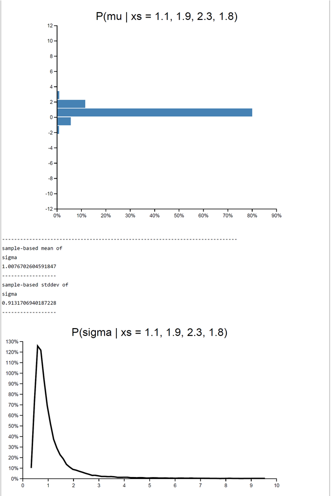
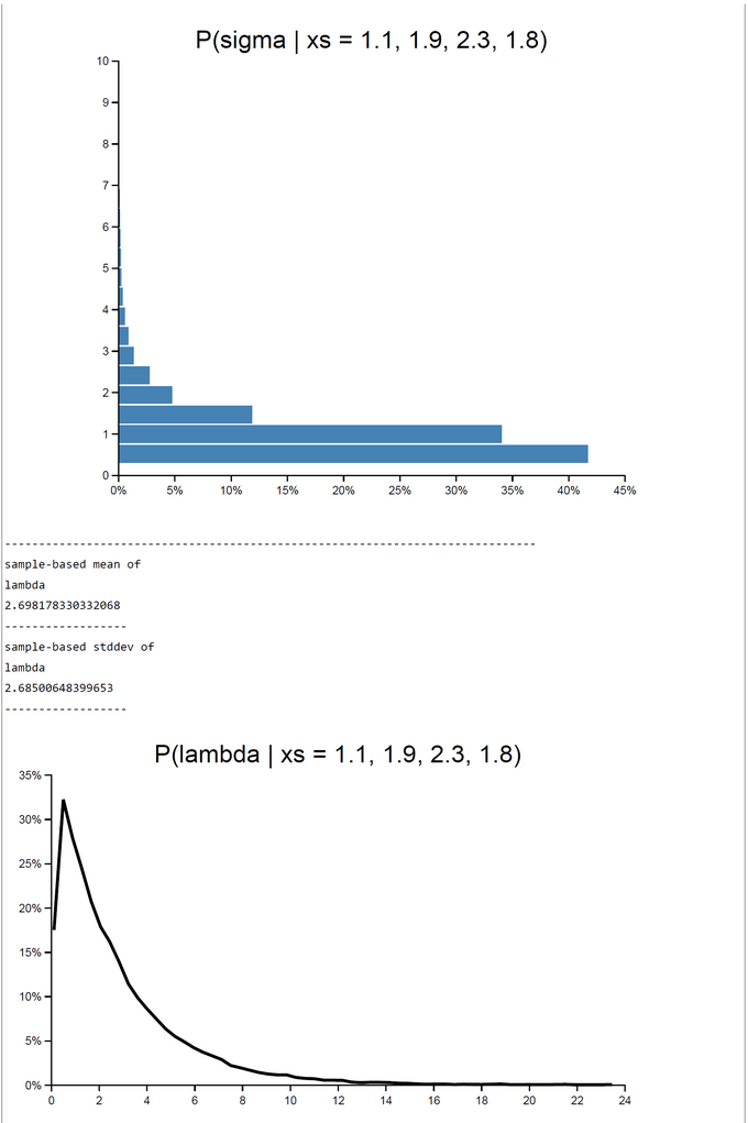
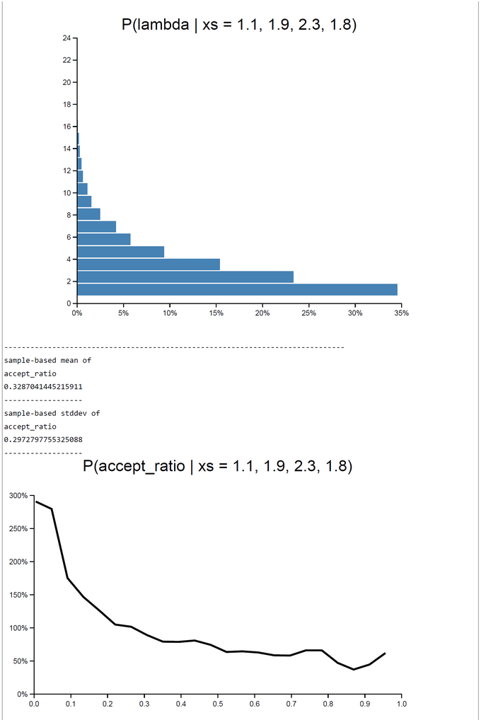
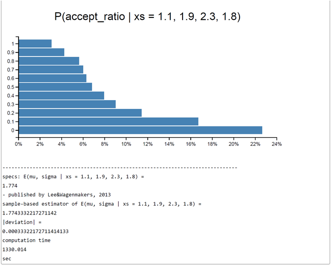
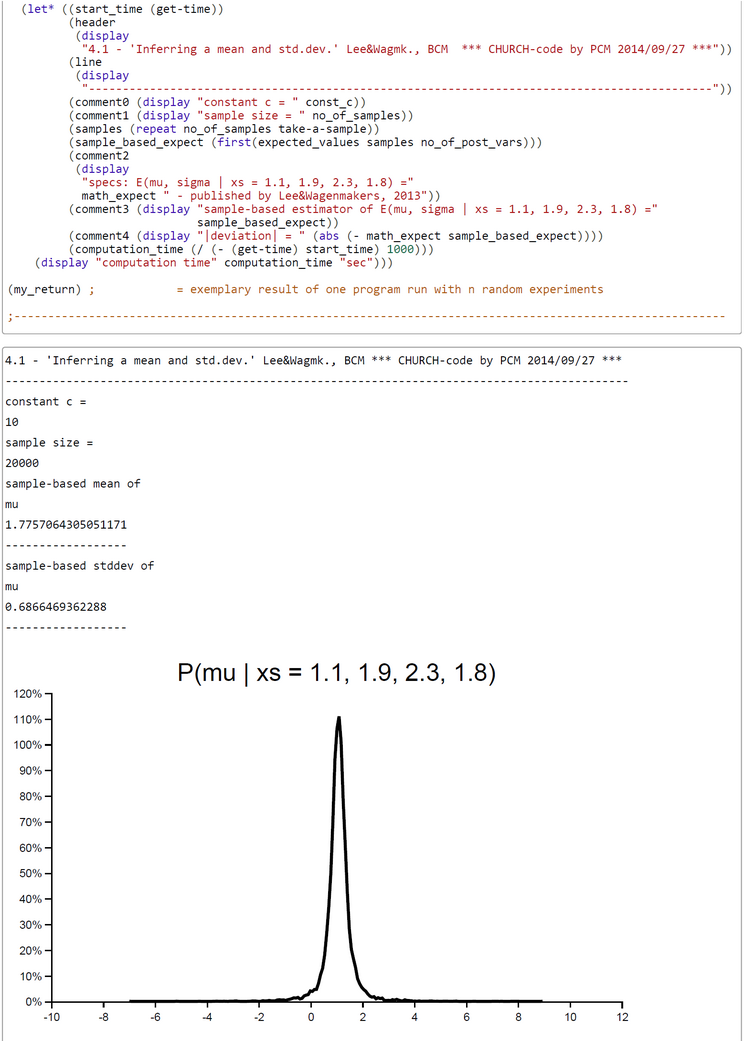
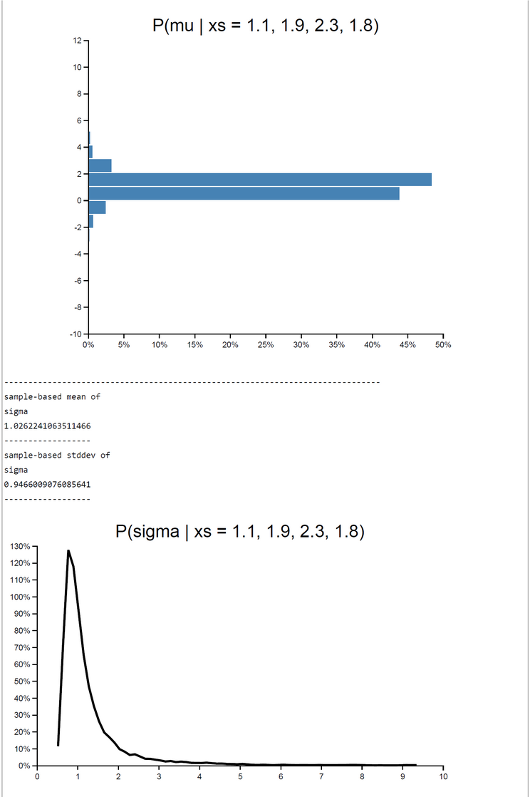
The method works excellent. The number of samples taken was set to 20000 in this run. This number could in principle be increased to get a better precision of estimates. The expected E(P(Acc)) was 0.3287041445215911. The WebChurch results for this problem agree nearly perfect with the OpenBUGS results: the absolute value of deviation between mean posterior mu is |deviation| = 0.00033322172711414133.
As a result we can say that computations programmed as as scripts within WebCHURCH are more concrete and under control of the modeller as their counterparts in OpenBUGS.
The screen-shots presented were generated by using the PlaySpace environment of WebCHURCH.
BCM-Ch04.1: CHURCH-Code for Rejection-Based Sampling with different mean Probabilities of Acceptance
The rationale why this rejection sampling with its 'soft' decision criterion P(Acceptance) = f(acceptance-ratio) works correctly can be found here (Albert,J., 2009, Bayesian Computation with R, Heidelberg: Springer, 2009, 2/e, ch.5.8, p.98f, DOI 10.1007/978-0-387-92298-0):
"A general-purpose algorithm for simulating random draws from a given probability distribution is rejection sampling. In this setting, suppose we wish to produce an independent sample from a posterior density g(theta | y) where the normalizing constant my not be known. The first step in rejection sampling is to find another probability density p(theta) such that:
- It is easy to simulate draws from p.
- The density p resembles the posterior density of interest g in terms of location and spread.
- For all theta and a constant c, g(theta | y) <= cp(theta).
Suppose we are able to find a density p with these properties. Then one obtains drwas from g using the following accept/reject algorithm:
- Independently simulate theta from p and a uniform random variable U on the unit interval.
- If U <= g(theta | y) / (cp(theta)), then accept theta as a draw from the density g; otherwise reject theta.
- Continue steps 1 and 2 of the algorithm until one has collected a sufficient number 'accepted' theta."
We define the 'probability of acceptance' P(Acc) = g(theta | y) / (c*p(theta)) <= 1. We decompose g(theta | y) into the product of likelihood and prior divided by a constant Z :
P(Acc) = g(theta | y) / [c*p(theta)] = ([p(y|theta)*q(theta)] / [Z*c*p(theta)]) <= 1.
Now we instantiate p(theta) by the prior q(theta) and c' by the product Z*c:
P(Acc) = ([p(y|theta)*q(theta)] / [Z*c*p(theta)]) = ([p(y|theta)*q(theta)] / [c'*q(theta)]) <= 1.
we can cancel q(theta):
P(Acc) = [p(y|theta) / c'] <= 1.
Our choice of a constant c' is only constrained by the above inequality. If c' is smaller than p(y|theta) then the acceptance ratio would be greater than 1. If c' is too big then P(Acc) will be too small and the sampling process will become inefficient though the results will still be unbiased and consistent.
A guess for c' is intuitive, when we instantiate p(y|theta) by the likelihood:
P(Acc) = [ L(y | theta ~ q(theta)) / c' ] <= 1.
Because the maximum-likelihood is greater or equal than any likelihood value L(y | theta ~ q(theta)) we can choose for c' the product [ c'' * L(x1,...,xn | mu = x-bar, sigma = s)] with c'' >=1 :
P(Acc) = [ L(y | theta ~ q(theta)) / (c'' * L(x1,...,xn | mu = x-bar, sigma = s))] = [ exp(ln L(y | theta ~ q(theta) - ln c'' - ln L(x1,...,xn | mu = x-bar, sigma = s))] <= 1.
In the code c'' is written constant_c. So we rename here c'' as c.
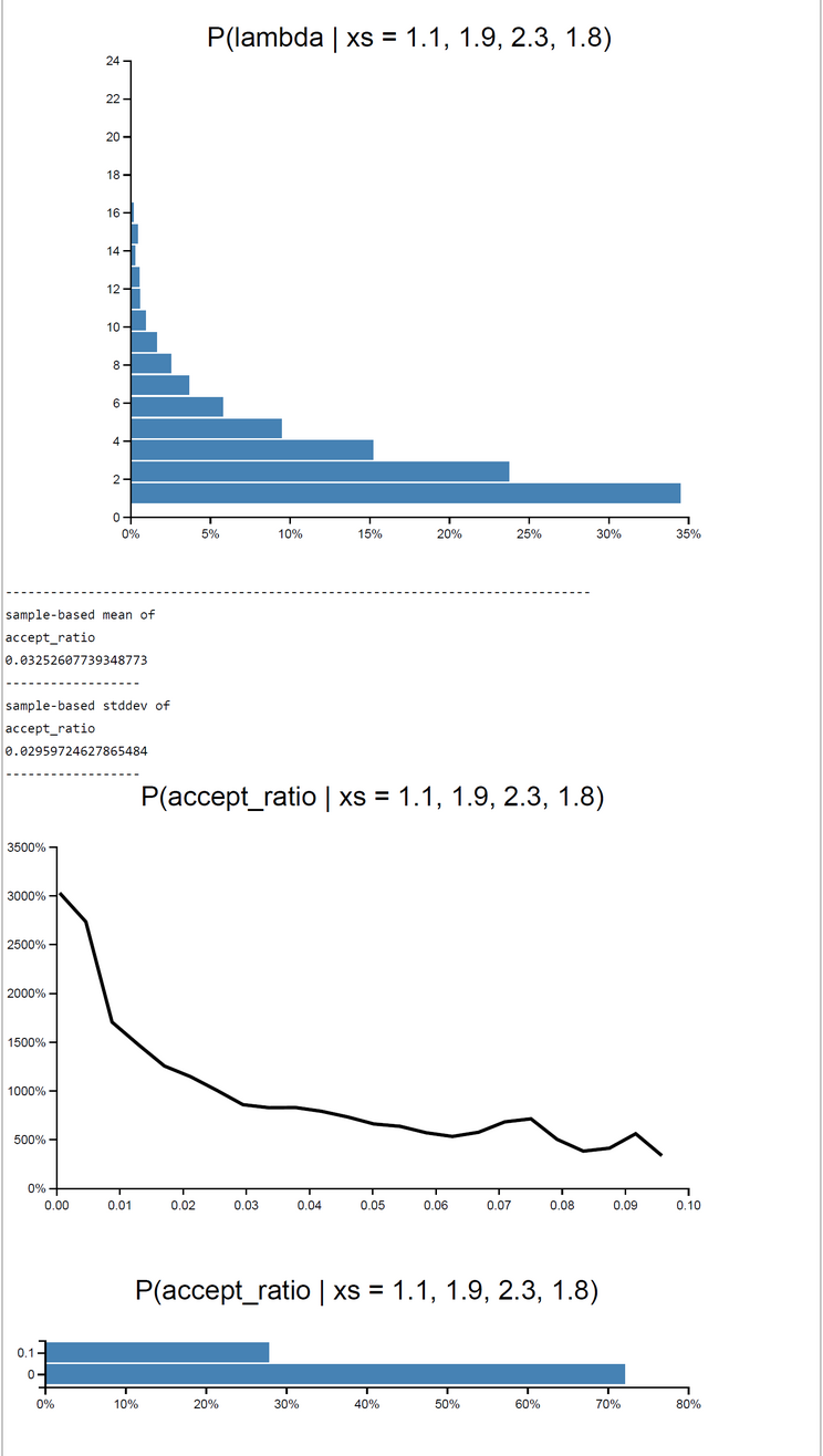
We made a small study how different values of c influenced the mean acceptance probability and total computation time. The sample size was fixed to N = 2000.
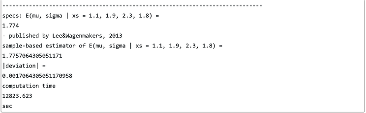
When c=1 rejection sampling is most efficient: E(P(Acc)) = 0.33395. For 2000 samples it took 162.55 sec to get the posterior pdfs. The mu-|deviation| = 0.01400. For greater c (c=10) the E(P(Acc)) drops down to 0.03252. At the same time computation time increases to 12823.623 sec. Despite the drop of E(P(Acceptance)) the deviation |mu_OpenBUGS - mu_WebCHURCH| remains stable: |deviation| = 0.00170. The table of results and the screenshot of this run with c = 10 can be found below.
| Platform | contant c | mean mu | |dev| | sd mu | mean sigma | sd sigma | E(P(Acc)) | seconds |
|---|---|---|---|---|---|---|---|---|
| OpenBUGS | 1.774 | 0.0000 | 0.6712 | 1.0100 | 0.9193 | |||
| WebCHURCH | 1 | 1.788 | 0.0140 | 0.5292 | 0.9782 | 0.8822 | 0.3339 | 162 |
| WebCHURCH | 2 | 1.746 | 0.0281 | 0.6205 | 1.0191 | 0.8853 | 0.1589 | 320 |
| WebCHURCH | 3 | 1.782 | 0.0076 | 0.6668 | 1.0182 | 0.9219 | 0.1079 | 3705 |
| WebCHURCH | 4 | 1.770 | 0.0036 | 0.6952 | 1.0210 | 0.9562 | 0.0816 | 5084 |
| WebCHURCH | 5 | 1.777 | 0.0033 | 0.6696 | 1.0193 | 0.9302 | 0.0650 | 6150 |
| ... | ||||||||
| WebCHURCH | 10 | 1.776 | 0.0017 | 0.6866 | 1.0262 | 0.9466 | 0.0325 | 12823 |
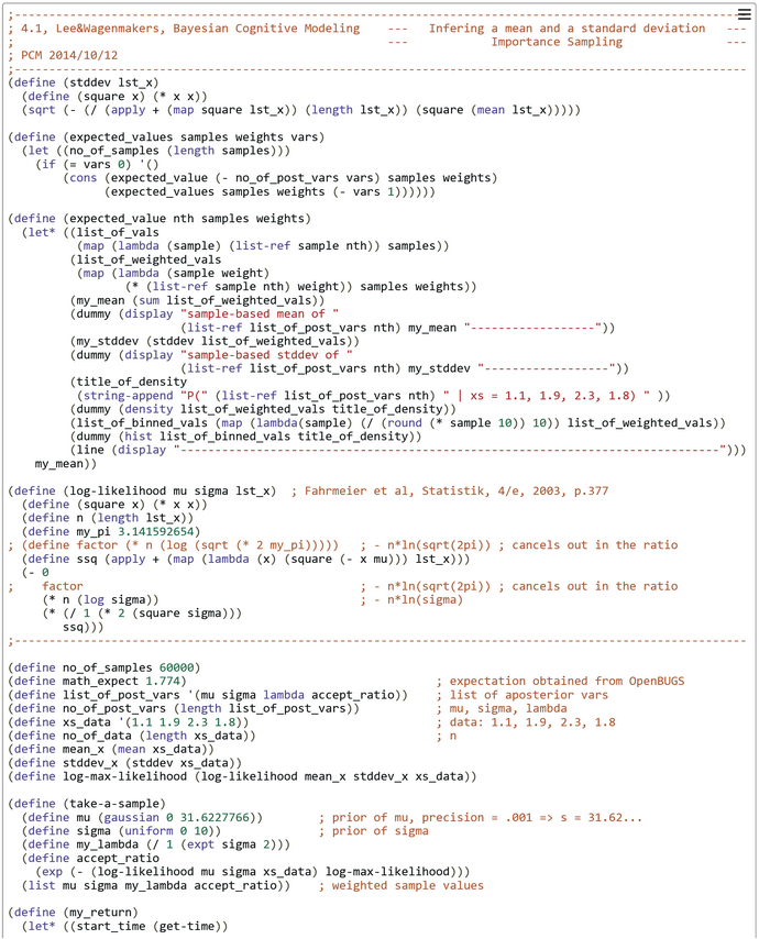
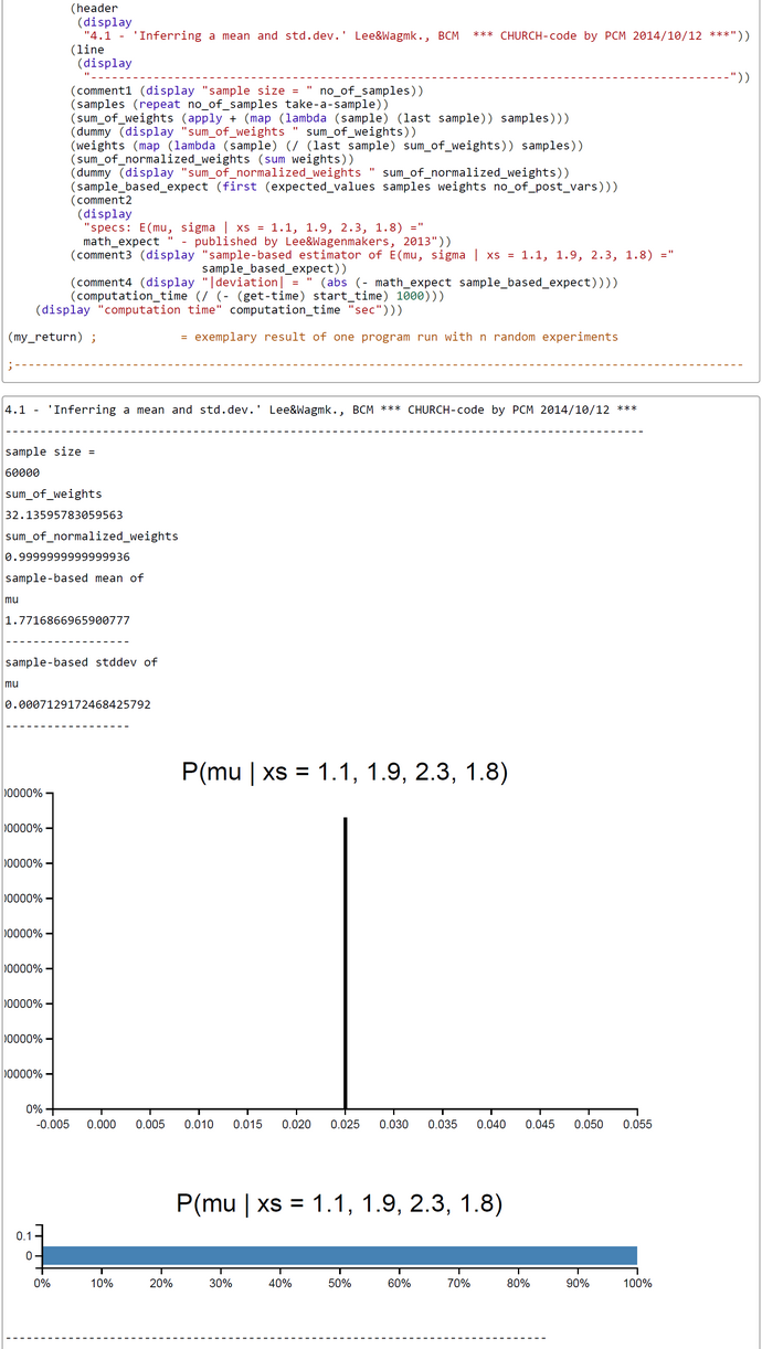
BCM-Ch04.1: CHURCH-Code for Importance-Based Sampling when "Inferring a mean and a standard deviation"
"In the situation where the posterior distribution is not a standard functional form, rejection sampling with a suitable choice of proposal density provides an alternative method for producing draws from the posterior. Importance sampling and sampling importance resampling (SIR) algorithms are alternative general methods for computing integrals and simulating from a general posterior distribution."(Albert, J., Bayesian Computation with R, 2009, 2/e, p.87f).
"In many situations, the normalizing constant of the posterior density g(theta | y) will be unknown, so the posterior mean of the function h(theta) will be given by the ratio of integrals:
E(h(theta) | y) = [Int(h(theta)*g(theta)*f(y|theta)dtheta] / [Int(g(theta)*f(y|theta)dtheta],
where g(theta) is the prior and f(y|theta) is the likelihood function. ... In the case where we are not able to generate a sample directly from g, suppose instead that we can construct a probability density p that we can simulate and that approximates the posterior density g. We rewrite the posterior mean as
E(h(theta) | y) = [Int(h(theta)*[g(theta)*f(y|theta)/p(theta)]*p(theta)dtheta] / [Int([g(theta)*f(y|theta)/p(theta)]*p(theta)dtheta] = [Int(h(theta)*w(theta)*p(theta)dtheta] / [Int(w(theta)*p(theta)dtheta,
where w(theta) = g(theta)*f(y|theta)/p(theta) is the weight function. If theta(1), ... , theta(m) are simulated sample from the approximation density p, then the importance sampling estimate of the posterior mean (of a function h(theta)) is:
h-bar_IS = Sum[h(theta(j)) * w(theta(j)); j=1,...,m] / [Sum[w(theta(j)); j=1,...,m]].
This is called an importance sampling estimate because we are sampling values of theta that are important in computing the integrals in the numerator and denominator." (Albert, J., Bayesian Computation with R, 2009, 2/e, p.101f).
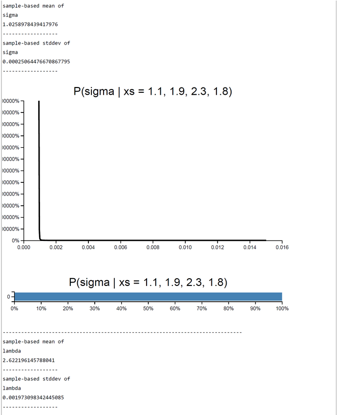
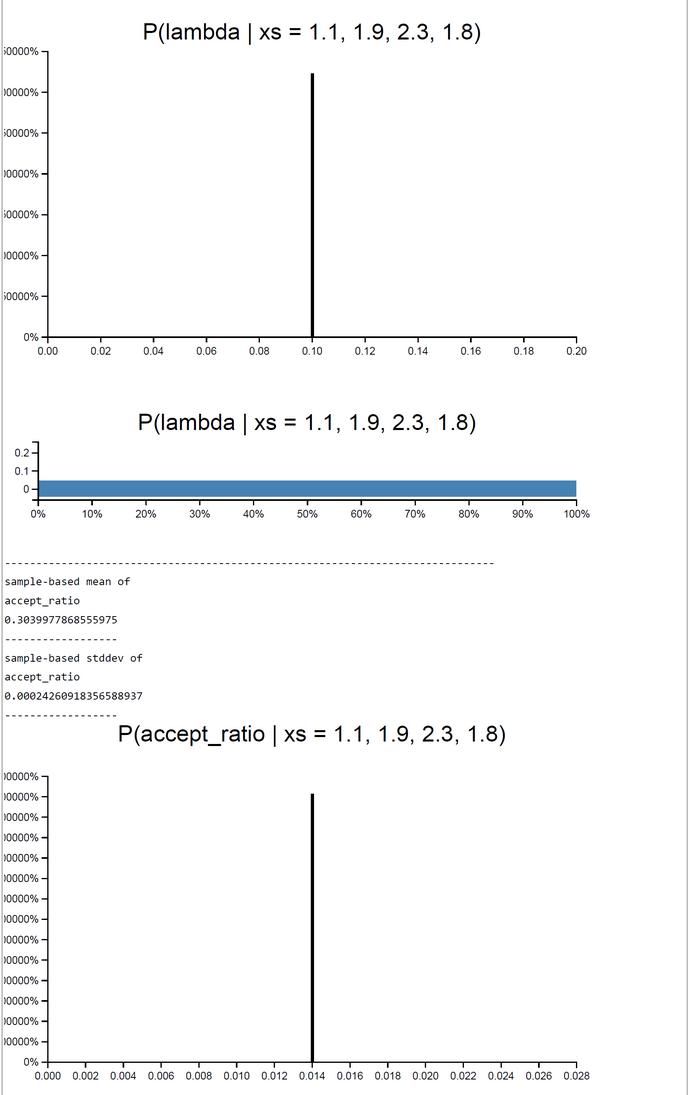
In our case we set h(theta(j)) = theta(j) and p(theta) = g(theta)*f_max(y|theta), where f_max(y|theta) is the maximum likelihood. In short, our weights w(theta) are the unnormalized accept-ratios or acceptance probabilities from rejections sampling (before) or MCMC (later). This is a nice result and works fine, as can be seen from the simulation run with 60.000 samples (below). The sample-based estimates corresond to those of rejection sampling and MCMC. The Church code can be found here.
BCM-Ch04.1: CHURCH-Code for MH-Based Sampling when "Inferring a mean and a standard deviation"
The signature of MH-Query as we used it is - with some minor modifications - taken from the old CHURCH documentation:
(mh-query samples lag defines query-expr condition-expr)
- normal-order evaluation.
- Do inference using the Metropolis-Hastings algorithm (as described in Goodman, et al., 2008).
- samples: The number of samples to take.
- lag: The number of iterations in between samples ('thin factor' in OpenBUGS-terminology).
- defines …: A sequence of definitions (usually setting up the generative model).
- query-expr: The query expression (the value or list of values sampled by each sample).
- condition-expr = boolean-expr | (condition boolean-expr) | (factor log(target-function))
- boolean-expr: Church-expression with a boolean value.
- MH-QUERY returns: A list of samples from the conditional distribution.
The cond-expr in the CHURCH-code of this example does not contain a 'hard' boolean expression as the ProBMod-Tutorial recommends. Instead it contains a 'soft' boolean constraint in the form of function call '(factor x)' where x is the log(target-function). The target-function is proportional to the Bayesian posterior, which is the product of the likelihood times the priors.
The use of '(factor x)' is an undocumented hack. The meaning of '(factor x) is equal to '(flip (exp x))'.
The most important function is 'take-samples'. It contains the Bayesian model. The WebChurch-code can be found here.
The simulation run is parametrized with a burnin-period of 20% the sample size N. The sample size is the number of samples after thinning out. We set the sample size to N = 10.000 so that the length of the burnin-period is 2000. The effective sample-size is N - length(burnin-period) = 8.000. One run with Lag=1 produced a slow falling ACF(Lag) (first graphic below). So we set the thin-factor to 200 (!). The ACF(Lag) now has no trend. So we think that thin-factor 200 is perfect. The simulation results are very close to the OpenBugs results:
| OpenBugs | WebChurch | |
|---|---|---|
| posterior mu | mean=1.774 (stdd=0.67) | mean=1.7704 (stdd=0.72) |
| posterior sigma | mean=1.01 (stdd=0.92) | mean=1.0214 (stdd=0.94) |
| posterior lambda | mean=2.711 (stdd=2.69) | mean=2.6744 (stdd=2.65) |
The absolute value of the deviation between the posterior mu and the empirical mean ist 0.004565. The computation time on a standard Windows PC seems with 342 seconds rather high, but we have to keep in mind that due to the high thin-factor of 200 the total of MH-steps is N*200 = 2.000.000.
Thus there are 5850 MH-steps/sec.


