Latent Class Mixture Model with Dirichlet Allocation
Latent Class Mixture Model with Dirichlet Allocation
Purpose of Model
The overall purpose of the model is to identify the underlying latent classes of a set of i.i.d. binomial distributed frequency counts. These frequencies could be the number of a set of i.i.d. bernouilli distributed 0-1, no-yes, false-true answers to test or questionionaire item.
The model is designed (1) to detect the number ng of latent classes, (2) to estimate the group-specific ability parameter to generate 'true' or 'yes' responses, (3) to identify for each of the n subjects the class zmax[i] with the greatest membership probability, (4) to estimate the person-specific ability parameter theta[i] to generate 'true' or 'yes' responses, and (5) the person-specific parameter theta[i] should be a mixture of the group-specific ability parameters ability[g], where the person-specific class-membership probabilities z[i,g] are the mixture coefficients.
BUGS-Code for Models with two or three Hypothized Latent Classes and Latent Dirichlet Allocation (LDA)
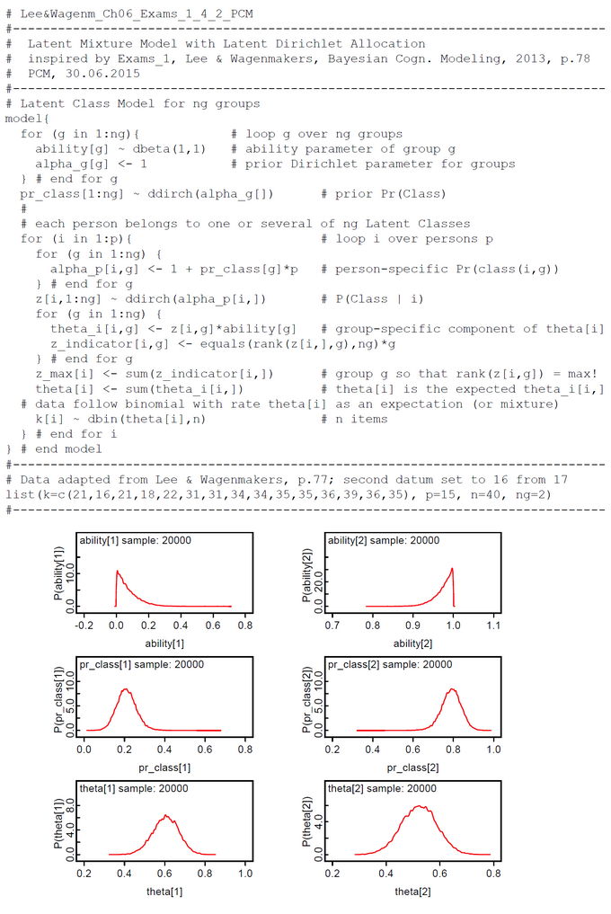
This is a code walk-through. The group-specific ability parameters ability[g] are sampled from a beta distribution with priors from a beta(1,1) which is a uniform(0,1). These samples are constrained like conventional probabilities: 0 <= ability[g] <= 1 and sum(ability[]) = 1.
The class membership probabilities pr_class[g] are sampled from a Dirichlet distribution with priors alpha_g[g] = 1. This is a multivariate generalization of the beta(1,1). This means that we assume, that all membership probabilities are samled from a maximal uninformed prior.
For each person i we sample a set class membership probabilities z[i,1:ng] from a Dirichlet distribution with priors which are biased by the class membership probabilities pr_class[g] and the total number of subjects p.
Next we compute the person-specific ability parameter theta[i] as an expected value of the group-specific ability parameters ability[g]. Mixture coefficients are the person-specific class-membership probabilities z[i,g]. As a side effect we get the class membership z_max[i] for person i which is the group g whith highest z[i,g].
The third last line of the program describes that the frequency count k[i] of person i is a binomial distributed variable with person-specific ability parameter theta[i] and n, which denotes the number of items.
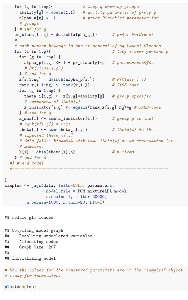
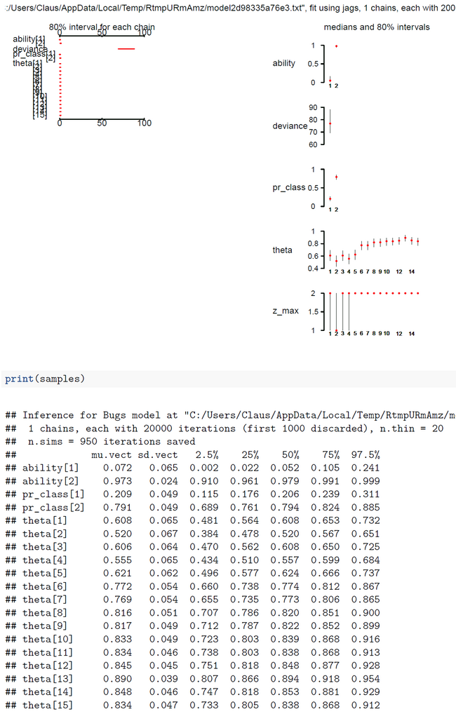
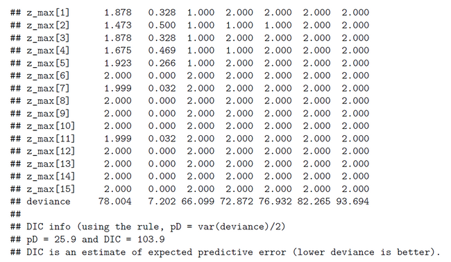
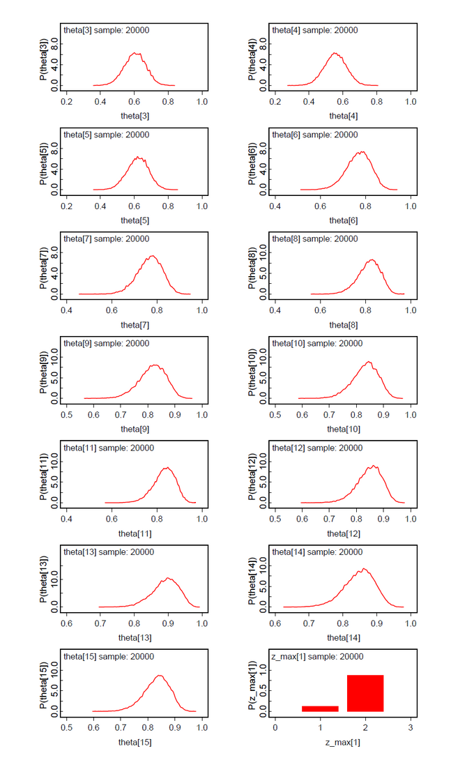
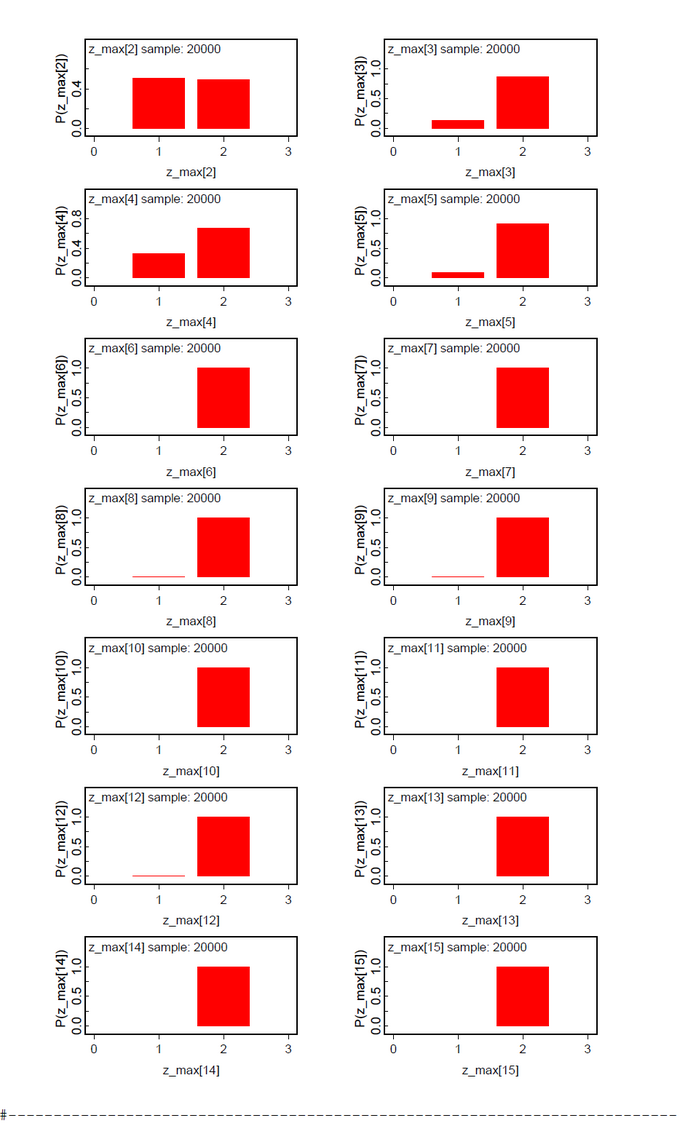
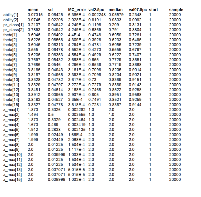
The first data set contains the original data from Lee & Wagenmakers Exam Scores problem but one exception. The second datum is changed from 17 to 16 to make the results more concise. We assume two latent classes (ng = 2). To our surprise the ability parameters have a tendency toward the extremes (Fig.01). There is a low tendency group 1 with mean(ability[1] ) = 0.0732 and Pr(Class=1)=0.2107 and a high tendency group 2 with mean(ability[2] ) = 0.9745 and Pr(Class=2)=0.7893 (Fig.04). By mixtures both ability parameters generate the person-specific ability parameters theta[i]. Pr(Class) and all theta[i] are within our expectations. When we look at the class assignments z_max (Fig.02-03) we see that subjects 6-15 are classified without any doubt into latent class 2 (high tendency class). The classification of subjects 1-5 is done with uncertainty. All these subjects (except subject 2) have a higher classification probability for class 2 but at the same time a nonzero proability for class 1. Now we see the reason that we diminished the score of subject 2.
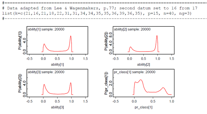
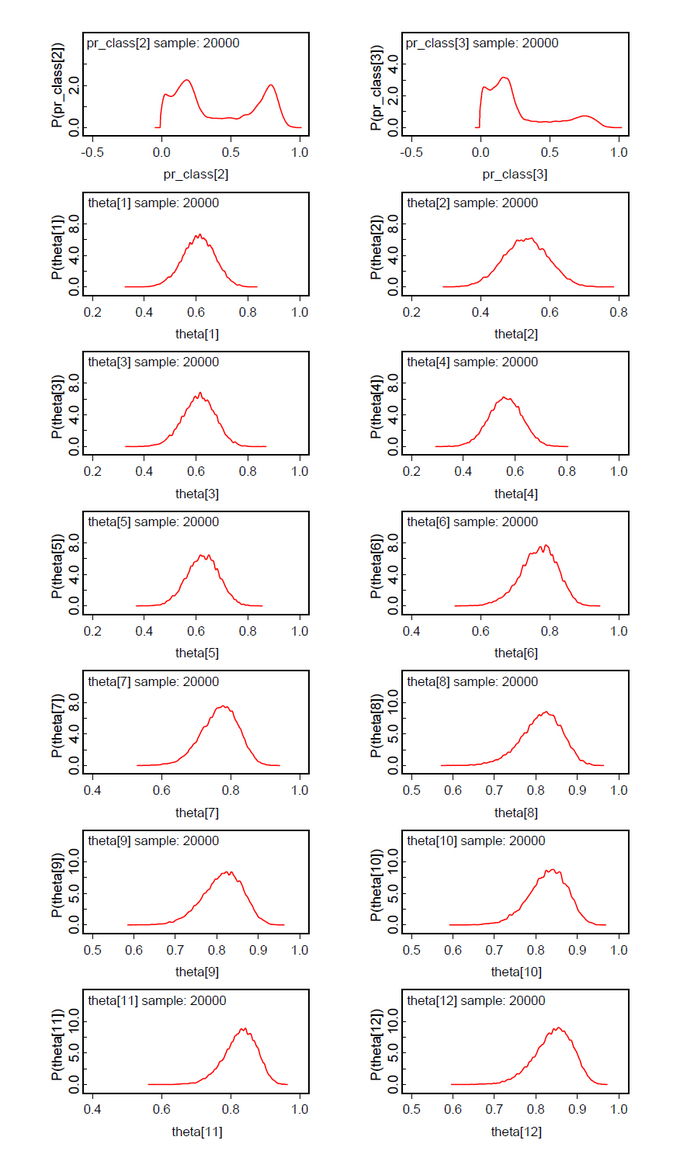
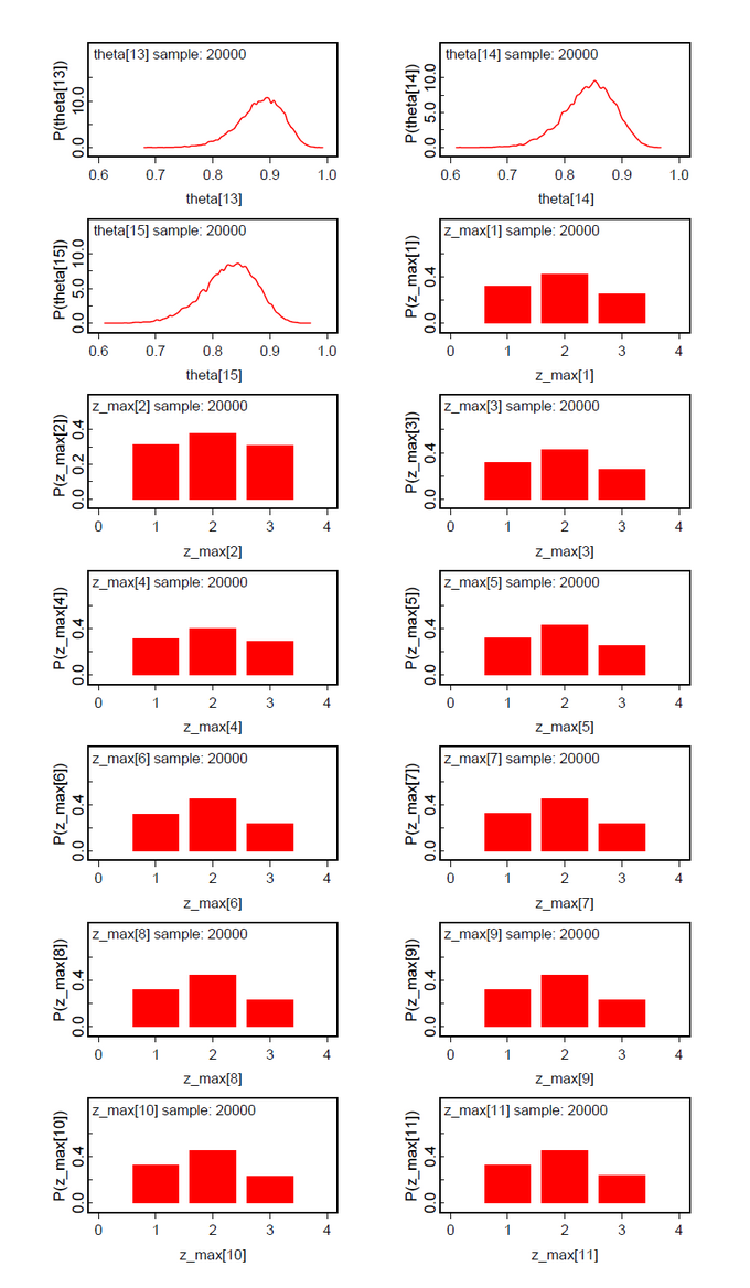
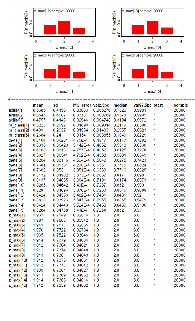
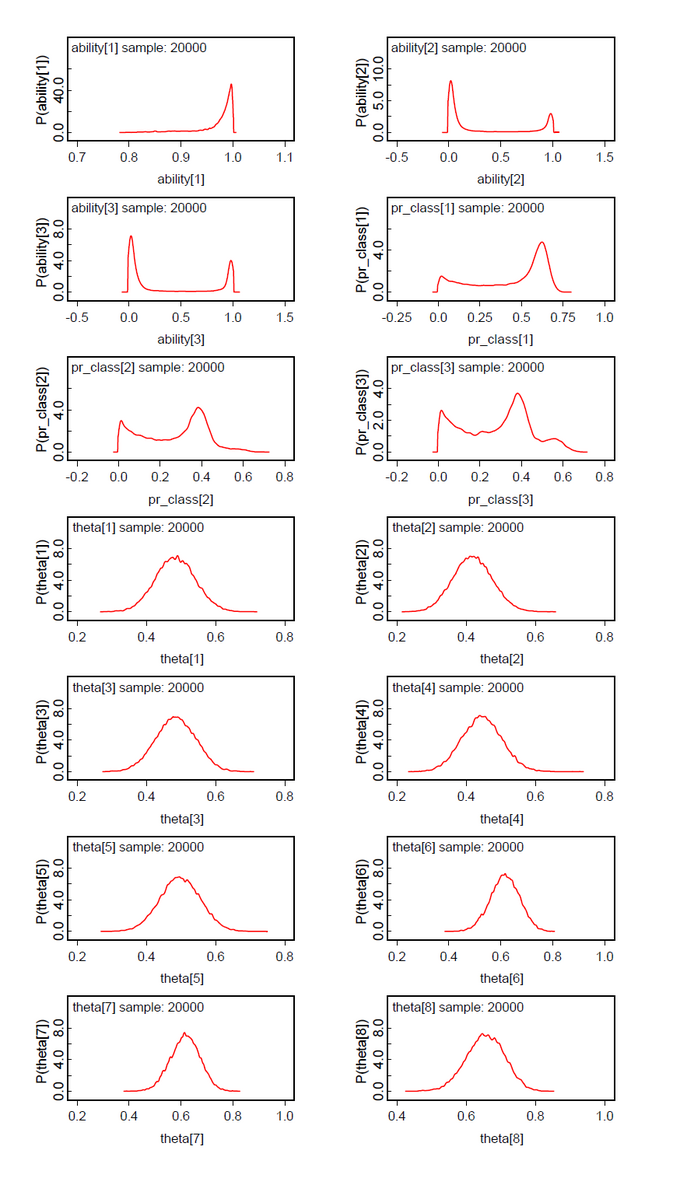
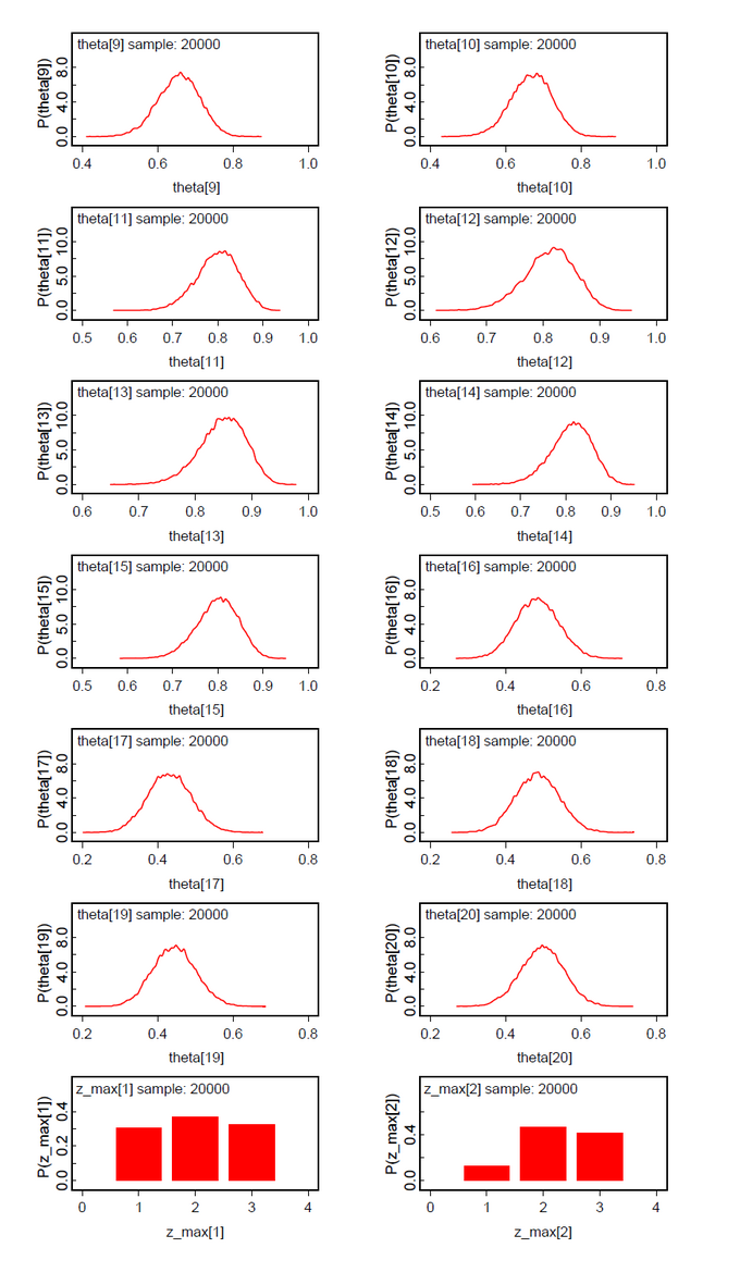
When we analyze the same data set under the assumption of ng=3 latent classes, the posteriori distribution of the ability parameters are bimodal with nearly the same shape (Fig.05). We suspect that the hypothesis of ng=3 should be abandoned in favor of ng=2. The class assignments z_max[i] support this conclusion by no clear class preference besides class 2.
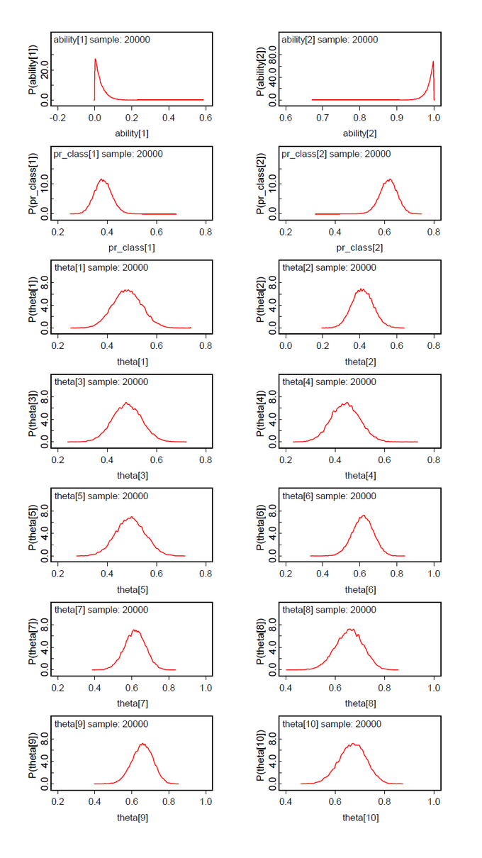
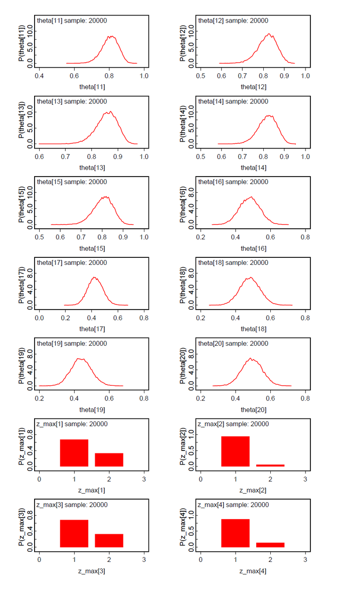
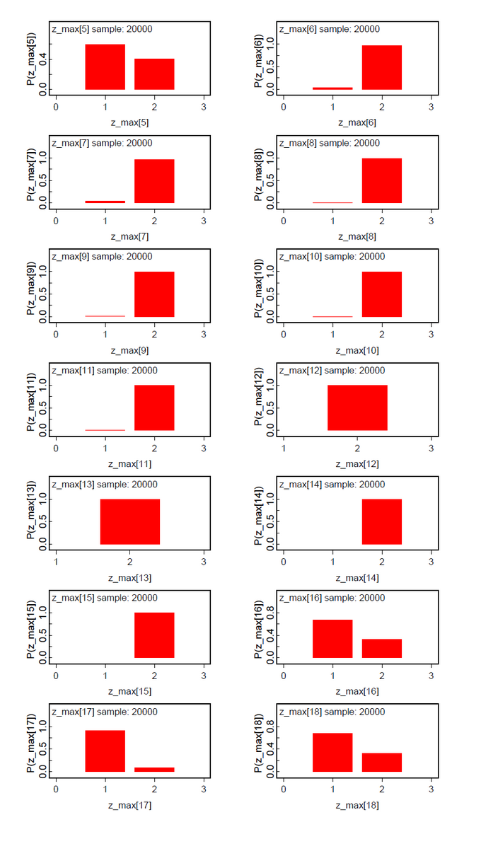
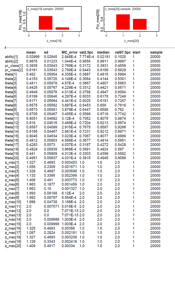
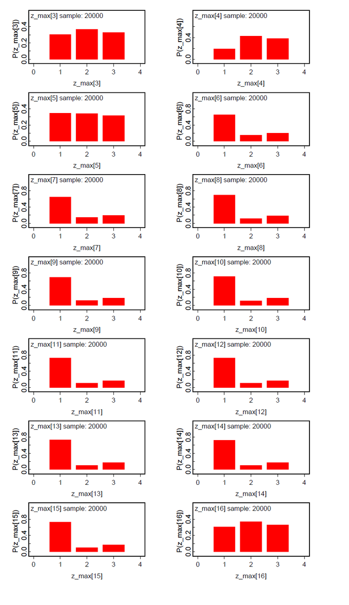
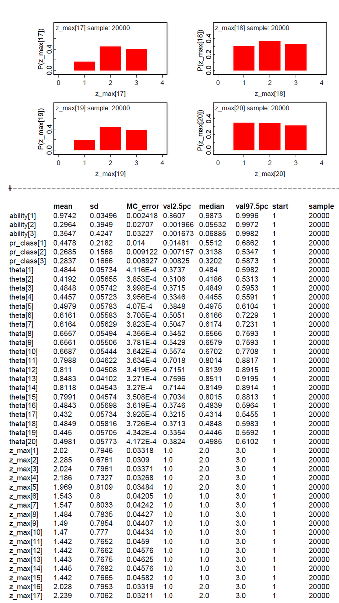
A second data set was generated by copying the first five data, adding 10 to n and to the data of subjects 11-15. From our intuition we would expect three classes Pr(Class=1)=0.50, Pr(Class=2)=0.25, and Pr(Class=3)=0.25.The results (Fig.09-13) demonstrate the clear separation of two latent classes.
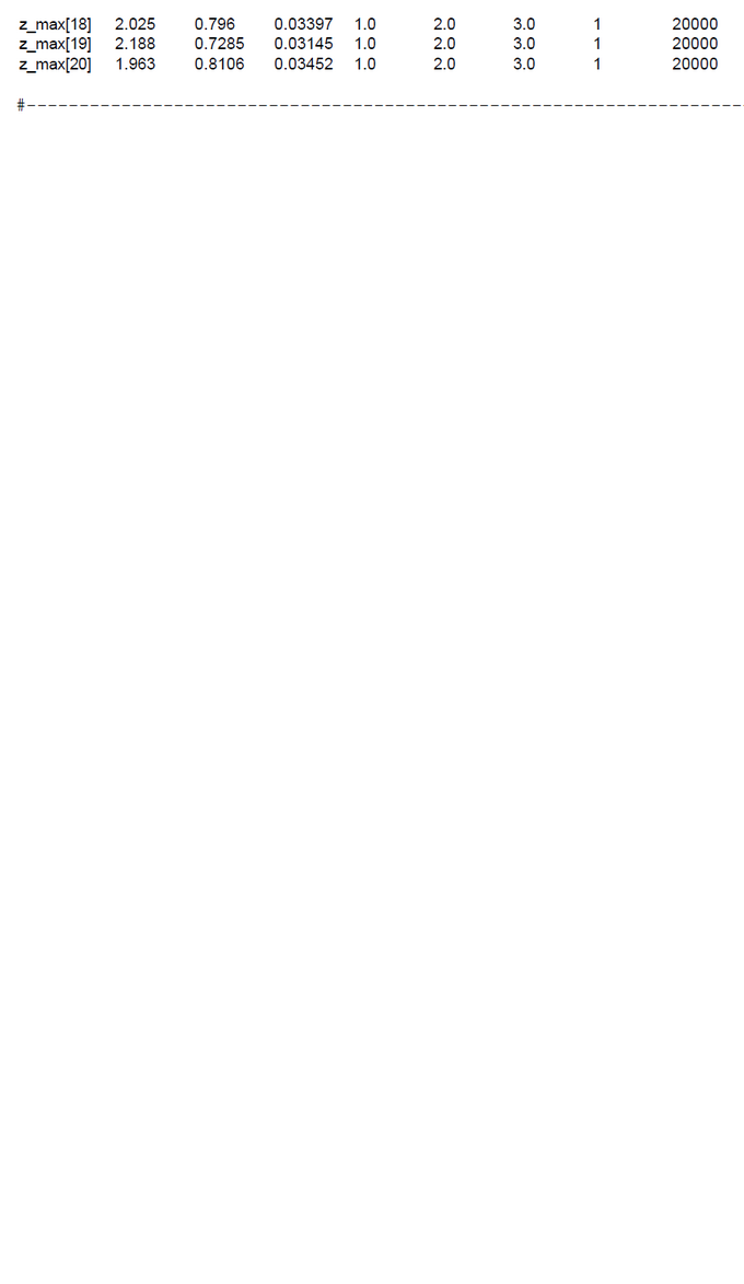
The same is true for the analysis of the same data set under the hypothesis ng=3 (Fig.14-19). The classes 2 and 3 could not be clearly discriminated. This means that subjects 1-5 and 16-20 belong to one latent class and subjects 6-15 to the other.
What has to be reflected is the Pr(Class). These results are not so clear cut. But as a summary the results are very promising.
To our knowledge this model is new. It does not need the EM-algorithm. In the next future we will study what is the relation between our model to the LDA-Topic Model (Blei, D.M.; Ng, A.Y.; Jordan, M.I.; Lafferty, J.; Latent Dirichlet Allocation, Journal of Machine Learning Research, 3 (4-5), pp. 993-1022).


JAGS-Code for Models with two or three Hypothized Latent Classes and Latent Dirichlet Allocation (LDA)
Various authors prefer JAGS to BUGS (e.g. Kruschke, J.K., Doing Bayesian Data Analysis, 2015, 2/e, Academic Press, ISBN 978-0-12-405888-0). The main differences are described in Lunn et al. in chapter 12.6 (Lunn, D.; Jackson, Chr.; Best, N.; Thomas, A., Spiegelhalter, D.; The BUGS Book: A Practical Introduction to Bayesian Analysis, Boca Raton, FL USA: CRC Press, 2013, ISBN 978-1-58488-849-9). We wanted to explore whether there are significant differences in modelling. We found out that are subtle differences in the modelling languages. The R-integration of JAGS is better than that of OpenBUGS. Models can be described as a user-defined parameterless R-function. So all editing, debugging and testing can be done with the excellent R-IDE RStudio.
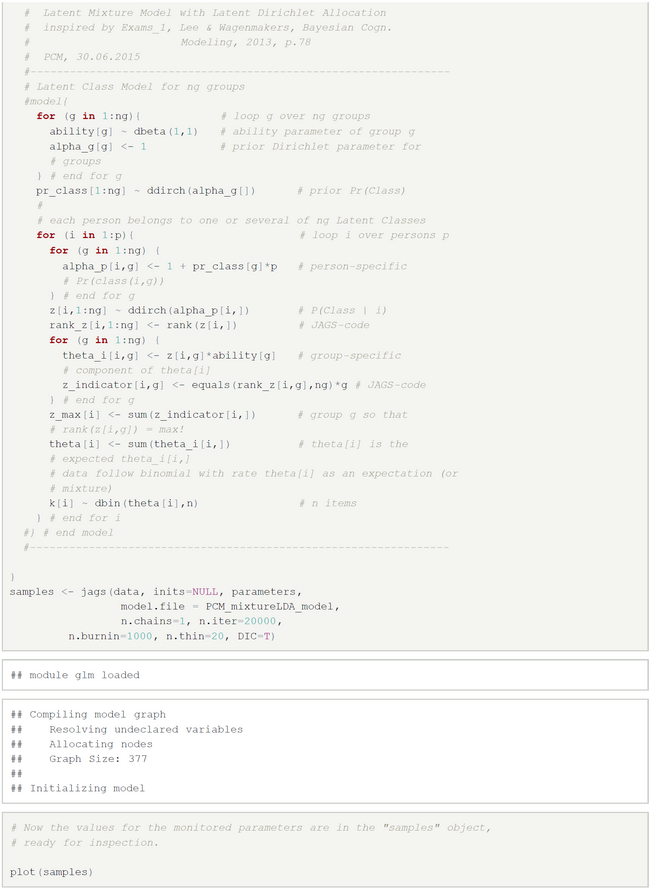
We had to revise our OpenBUGS-model in three places: (1) we replaced the model{...} BUGS-code-snippet by the R-code-snippet function(){...}; (2) because the definition of rank(...)-function differ in BUGS and JAGS we had to recode the computation of the class assignment z_max[]; (3) all data are encoded as R-statements and used as arguments in the jags-function of the R2jags-library.
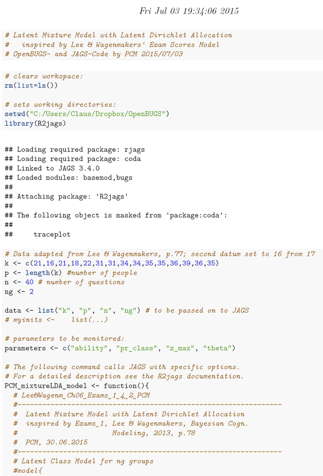
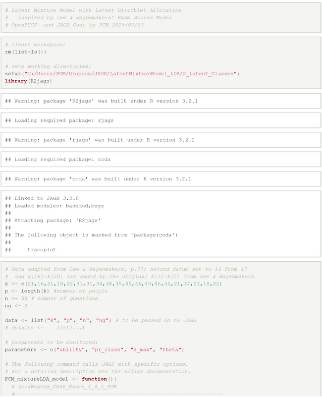
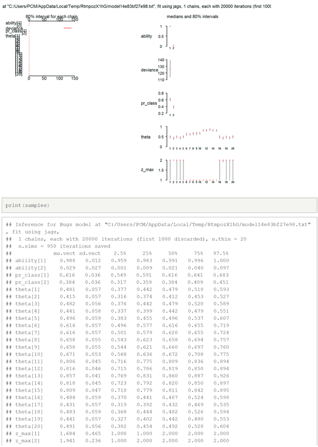
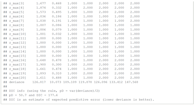
The results for two latent classes and the slightly modified data of Lee & Wagenmakers (k[2]=16 instead of 17, 15 subjects, 40 items) are nearly identical to those of the OpenBugs analysis (Fig.01-04). The means of the posteriors for abilities and class probabilities differ only by 0.08.
Nearly the same is true for the slightly modified problem ((k[2]=16 instead of 17, k[16]-k[20] added, 20 subjects, 50 items) (Fig.05-08).
