Pi by Monte-Carlo-Simulation
Pi by Monte-Carlo-Simulation
Pi by Monte-Carlo-Simulation
"Monte Carlo methods vary, but tend to follow a particular pattern:
- Define a domain of possible inputs.
- Generate inputs randomly from a probability distribution over the domain.
- Perform a deterministic computation on the inputs.
- Aggregate the results.
For example, consider a circle inscribed in a unit square. Given that the circle and the square have a ratio of areas that is π/4, the value of π can be approximated using a Monte Carlo method:[3]
- Draw a square on the ground, then inscribe a circle within it.
- Uniformly scatter some objects of uniform size (grains of rice or sand) over the square.
- Count the number of objects inside the circle and the total number of objects.
- The ratio of the two counts is an estimate of the ratio of the two areas, which is pi/4. Multiply the result by 4 to estimate pi.
In this procedure the domain of inputs is the square that circumscribes our circle. We generate random inputs by scattering grains over the square then perform a computation on each input (test whether it falls within the circle). Finally, we aggregate the results to obtain our final result, the approximation of π.
If the grains are not uniformly distributed, then our approximation will be poor. Secondly, there should be a large number of inputs. The approximation is generally poor if only a few grains are randomly dropped into the whole square. On average, the approximation improves as more grains are dropped." (Wikipedia, visited 2014/07/29)
CHURCH-Code for Pi-Monte-Carlo-Simulation
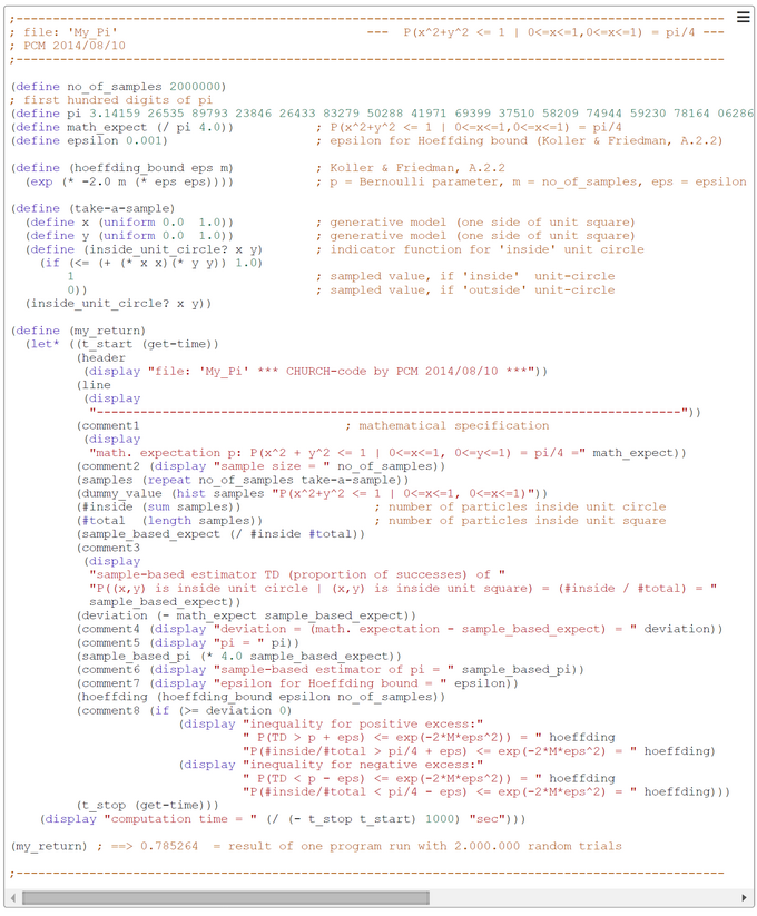
The Pi-Monte-Carlo-Simulation is well known and simulation code exists in various programming languages. We use the problem to demonstrate its solution in a functional CHURCH program (CHURCH is a probabilistic functional descendant of the general purpose language SCHEME).
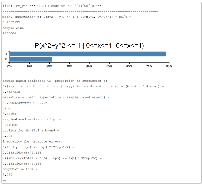
The generative model is contained in the CHURCH function "take-a-sample". The number of samples m was computed according to the Hoeffding bound (Koller & Friedman, Probabilistic Graphical Models, 2009, A2.2, p.1145). The Hoeffding bound guarantees that for a chosen m and epsilon the probability that the sample-based estimator TD (proportion of successes) deviates more than epsilon from the true Bernoulli-parameter p is less than the bound exp(-2*M*eps^2). For our application TD = #(particle (x, y) is within unit circle | particle (x, y) is within unit square) = #inside/#total.
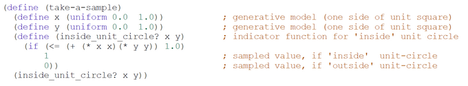
The sampling method used is the simple-to-understand 'forward sampling'. The screen-shot presented was generated by using the PlaySpace environment of WebCHURCH.
The code is self-explanatory. One random particle p = (x, y) falling within a unit square is generated. If it falls within the unit circle the sampled value is 1 otherwise 0. These values are collected in a list samples. The sum of samples is the number of particles #inside falling inside the unit circle. The length of samples is number of particles #total falling inside the unit square. The probability that the particle p is inside the unit circle is P(x^2 + y^2 <= 1 | 0 <=x<= 1, 0 <=y<= 1) = area_of_unit_circle_sector/area_of_unit_square = ((1/4)*pi*r^2)/r^2 = pi/4. This probability p = pi/4 can be estimated by the ratio #inside/#total. So pi = 4*p or approximately 4*(#inside/#total).