Example 9: Lotka-Volterra Dynamic Population Model
Example 9: Lotka-Volterra Dynamic Population Model
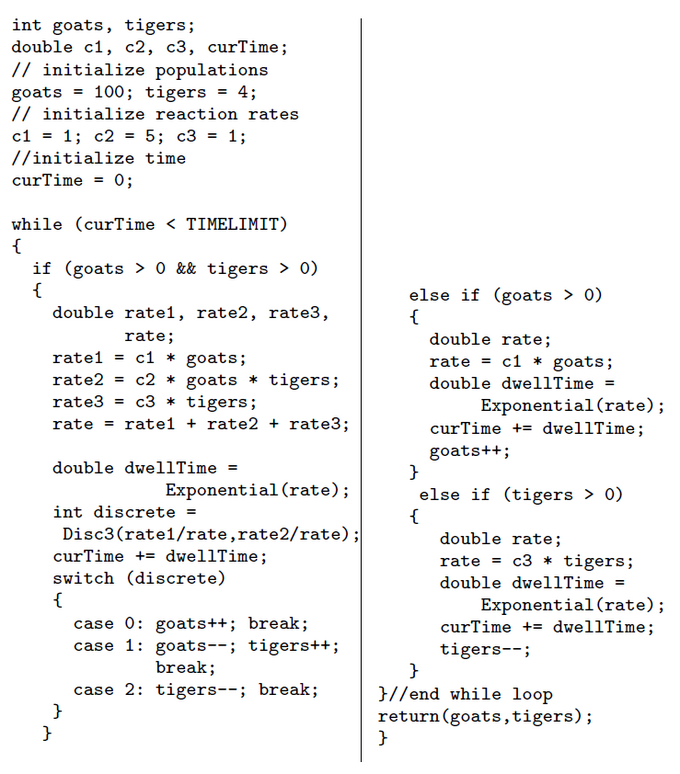
Example 9: Prob-C Code for the Lotka-Volterra Dynamic Population Model
In their overview article about probabilistic programming the authors present a series of paradigmatical examples (Gordon, Henzinger, Nori & Rajamani, Probabilistic Programming, 2014). Example 9 deals with the classical predator-prey population model known as Lotka-Volterra model. The convential model is formulated as system of deterministic differential equations. Here the authors offer a stochastic solution in form of a probabilistic C-like computer code (Prob-C). The underlying mathematical model is a Continous-Time Markov Chain (CTMC).
"The Lotka-Volterra predator-prey model (Lotka, 1925; Volterra, 1926) is a population model which describes how the population of a predator and prey species evolves over time. It is specified using a system of so called 'stoichiometric' reactions as follows:
$$G \longrightarrow 2G$$
$$G+T \longrightarrow 2T$$
$$T \longrightarrow 0$$
We consider an ecosystem with goats (denoted by G) and tigers (denoted by T). The first reaction models goat reproduction. The second reaction models consumption of goats by tigers and consequent increase in tigers. The third reaction models death of tigers due to natural causes.
It turns out that this system can equivalently modelled as a Continuous Markov Chain (CTMC) whose state is an ordered pair (G, T) consisting of the number of goats G and the number of tigers T. The first reaction can be thought of as a transition in the CTMC from state (G, T) to (G + 1, T) and this happens with a rate equal to $$c_1 \cdot G$$ where c1 is some rate constant, and is enabled only when G > 0. Next, the second reaction can be thought of as a transition in the CTMC from state (G, T) to (G-1, T+1) and this happens with a rate equal to $$c_2 \cdot G \cdot T $$, where c2 is some rate constant, and is enabled only when G > 0 and T > 0. Finally , the last reaction can be thought of as a transition in the CTMC from state (G, T) to (G, T-1) and this happens with a rate equal to $$c_3 \cdot T $$ where c3 is some rate constant, and is enabled only when T > 0.
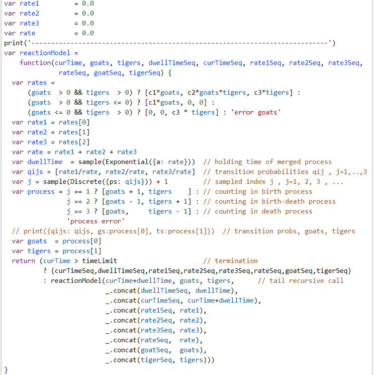
Using a process called uniformization, such a CTMC can be modeled using an embedded Discrete-Time Markov Chain (DTMC), and encoded as a probabilistic program, shown in Figure 1. The program starts with an initial population of goats and tigers and executes the transitions of the Lotka-Volterra model until a prescribed time limit is reached, and returns the resulting population of goats and tigers.
Since the executions are probabilistic, the program models the output distribution of the population of goats and tigers. The body of the while loop is divided into 3 conditions:
- The first condition models the situation when both goats and tigers exist, and models the situation when all 3 reactions are possible.
- The second condition models the situation when only goats exist, which is an extreme case, where only reproduction of goats is possible.
- The third condition models the situation when only tigers exist, which is another extreme case, where only death of tigers is possible." (Gordon et al., 2014, p.6)

Example 9: Formal Reconstruction of Gordon's et al. Prob-C Code
We think that the so called 'stoichiometric' reactions are misleading because they are rather different from chemical stoichiometric 'equations' or 'patterns'. According to Gordon et al. agent 'molecules' can appear out of nothing or disappear into nothing. This is not allowed in classical stoichiometry (Erban & Jonathan, 2020).
So we prefer to model the Lotka-Volterra-Scenario directly as a competitive Continuous Time Markov Chain (CTMC) with countable state space along its definition (e.g. Pishro-Nik, 2014, p.666; Ross, 2010, 10/e, p.373) with two subprocesses:
- a holding-time process, when in state i
- a jump process from state i to a different state j
Besides their standard use in natural (Erban & Chapman, 2020) and computational (Gordon, 2014; Mitzenmacher & Upfahl, 2018; Cassandras & Lafortune, 2008) sciences CTMCs are a non-standard modelling tool in psychology (Wickens, 1982, McGill, 1967; Diederich & Mallahi-Karai, 2020) and sociology (Coleman, 1964; Bartholomew, 1967; Tuma & Hannan, 1984).
The holding-time Poisson counting process is waiting for an event of type birth (of prey) or fatal attack (of predator), or death (of predator). In this kind of process it is assumed that holding or waiting times are exponential distributed with rates:
$$\lambda(G,T) = \lambda_1(G) +\lambda_2(G,T) + \lambda_3(T).$$
$$\lambda_1(G) = c_1 \cdot G \text{ ; birth process with birth events}$$
$$\lambda_2(G, T) = c_2 \cdot G \cdot T \text{ ; birth-death process with attack events}$$
$$\lambda_3(T) = c_3 \cdot T \text{ ; death process with death events}$$
Because rates are state-dependent the Poisson counting processes are inhomogeneous. The total rate is a sum of the rates of the three individual and independent Poisson counting subprocesses (birth, birth-death, and death) running parallel and in competion to each other. Poisson race processes are widely used in such diverse fields as cognitive reaction time (RT), choice processes or reliability studies (Ibe, 2013, ch. 2.7.5; 2014, ch. 12.5.9). In independent Poisson race processes the total rate is the sum of the rates of the subprocesses and the probability of winning this race can be determined by the ratio:
$$ p_{j} = \frac{\lambda_{j}}{\lambda} \text{ ; j = 1,...,3} \text{ ; probability of j is winning the process race}.$$
As the interarrival times of a Poisson counting process have an exponential distribution we can sample holding times ('dwellTime') of the merged Poisson process
$$ \Delta t(G, T) \sim DExp(\lambda(G,T)) = DExp('rate')$$
add them up to the current time ('curTime'), and compare the current time with our TIMELIMIT.
At the end of the holding-time interval the CTMC has to determine which of the three subprocesses generated the event. The probability of winning the race between the three Poisson counter processes and the jump-to probability is the simple standardized rate parameter (Ibe, 2013, ch. 2.7.5; 2014, ch. 12.5.9):
$$ p_{ij}(G,T) = \frac{\lambda_{ij}(G,T)}{\lambda_i(G,T)} \text{ ; i = 1, 2, ..., ; j = 1,...,3}.$$
Since the rates and probabilities for all i are constant ("uniform"), we suppress the state index i from now on.
$$ p_{j}(G,T) = \frac{\lambda_{j}(G,T)}{\lambda(G,T)} \text{ ; j = 1,...,3} \text{ ; probability that j is winning the process race}.$$
The jump-to index j is sampled from discrete distribution with the jump probabilities as parameter vector
$$j(G,T) \sim Discrete(p_1(G,T), p_2(G,T), p_3(G,T)) \text{ ; j = 1, ..., 3}$$
According to the selected jump-to index j the three processes generate at most two simultaneous actions. According to Gordon et al. these actions are:
$$(G, T) \stackrel{c_1 \cdot G}{\longrightarrow} (G+1, T) \text{ ; if j = 1, then birth process}$$
$$(G, T) \stackrel{c_2 \cdot G \cdot T}{\longrightarrow} (G-1, T+1) \text{ ; if j = 2, then birth-death process}$$
$$(G, T) \stackrel{c_3 \cdot T}{\longrightarrow} (G, T-1) \text{ ; if j = 3, then death process}$$
The simultaneous actions of the birth-death process (j = 2) are definitional for this kind of process, though they seem to be a bit unnatural in the Lotka-Volterra context. It is a bit unrealistic that during an exponential distributed attack episode a goat's disappearance is accompanied in the same episode by a birth of a tiger.
These transitions reach every state i in two-dimensional state-space S.
$$ S \subseteq G \times T $$ $$ G, T \subset \mathbb{N} $$
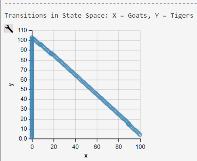
Transitions of the Lotka-Volterra CTMC are visualized in a transition-rate diagram (Fig. 2). This 2-dimensional transition space is typical for a competition process (Reuter, 1961; Iglehart, 1964) . It deviates from the conventional one-dimensional transition space typically used in CTMC definitions.
Empirical research has shown that the maximum of the predator frequency distribution appears most times later than the maximum of the prey distribution. This is not true for Gordon et al's model, when we use their rate-constants c as we demonstrate with our WebPPL-coded reconstruction (see below).
The classical Lotka-Volterra model is valuable for educational purposes but too too simple for empirical predictions and as an agent-based (
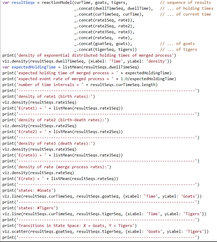
WebPPL-Implementation of the Lotka-Volterra Continous-Time Markov Chain (CTMC) Model
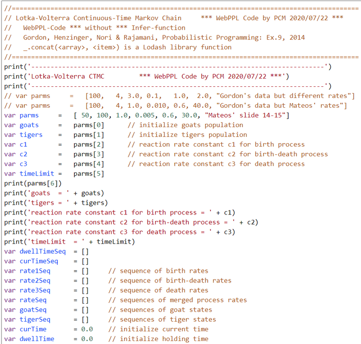
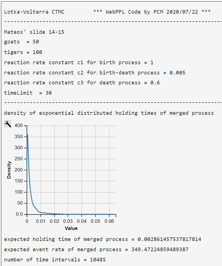
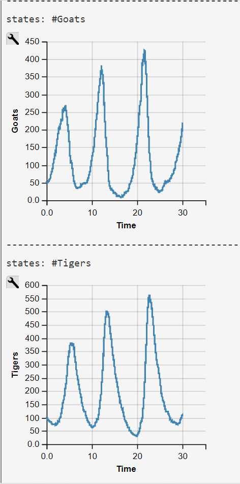
Lotka-Volterra Simulation Run with WebPPL Script and Mateos' Parameters
Mateos' parameters were obtained from his 2018 lecture slides (visited 2020/07/27)
$$c_1 = 1.0$$
$$c_2 = 0.005 $$
$$c_3 = 0.6 $$
$$Goats(0) = 50$$
$$Tigers(0) = 100 .$$
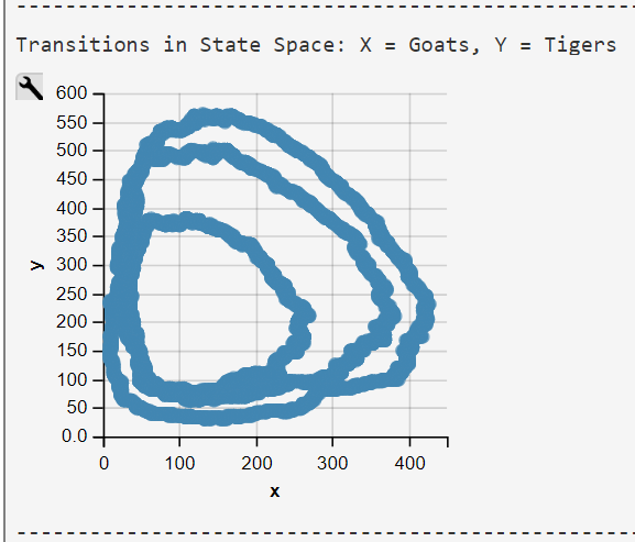
The WebPPL-Code was developed independently. Results are similar though some of our simulations runs end in an ex- or implosion of the state space.


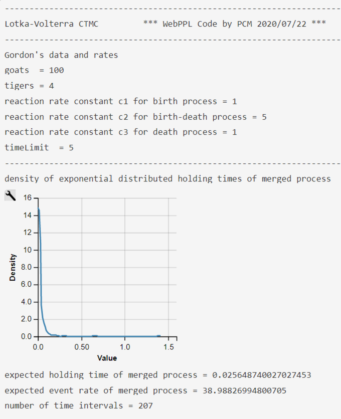
Lotka-Volterra Simulation Run with WebPPL Script and Gordon et al.'s Parameters and Rates
Gordon et al.'s parameters and rates were obtained from the authors 2014 publication (visited 2020/07/28).
$$c_1 = 1.0$$
$$c_2 = 5.0 $$
$$c_3 = 1.0 $$
$$Goats(0) = 100$$
$$Tigers(0) = 4 .$$
The pure functional WebPPL-Code is an independently developed reimplementation of the imperative Prob-C code . Results demonstrate that the model does not show the typical Lotka-Volterra behavior with its cyclic trajectories. A model run with Mateos' start parameters and rate are much more typical for the Lotka-Volterra model trajectories (see above).